Sentinel-1
Learning Objectives
A 30 minute guide to Sentinel-1 data for SnowEX
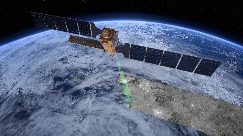
Fig. 6 Artist view of Sentinel-1. image source: https://www.esa.int/ESA_Multimedia/Images/2014/01/Sentinel-1_radar_vision)
See also
this tutorial is a quick practical guide and will not cover InSAR processing, check out UNAVCO InSAR Short Courses if you’re interested in learning custom processing of SAR data.
Dive right in
Synthetic Aperture Radar (SAR) is an active imaging technique that records microwave reflections off of Earth’s surface. Unlike passive optical imagers that require cloud-free, sunny days, SAR can operate at night and microwaves penetrate clouds At first glance, a SAR ‘image’ might look a lot like a black-and-white image of the Earth, but these observations contain more than just color values and can be used to query many physical properties and processes!
But before getting into theory and caveats, let’s visualize some data. An easy way to get started with Sentinel-1 SAR over a SnowEx field site is to use the Radiometric Terrain Corrected (RTC) backscatter amplitude data on AWS: https://registry.opendata.aws/sentinel-1-rtc-indigo/
# GDAL environment variables to efficiently read remote data
os.environ['GDAL_DISABLE_READDIR_ON_OPEN']='EMPTY_DIR'
os.environ['AWS_NO_SIGN_REQUEST']='YES'

# Data is stored in a public S3 Bucket
url = 's3://sentinel-s1-rtc-indigo/tiles/RTC/1/IW/12/S/YJ/2016/S1B_20161121_12SYJ_ASC/Gamma0_VV.tif'

# These Cloud-Optimized-Geotiff (COG) files have 'overviews', low-resolution copies for quick visualization
da = rioxarray.open_rasterio(url, overview_level=3).squeeze('band')
da.hvplot.image(clim=(0,0.4), cmap='gray',
                x='x', y='y',
                aspect='equal', frame_width=400,
                title='S1B_20161121_12SYJ_ASC',
                rasterize=True # send rendered image to browser, rather than full array
               )
Interpretation
The above image is in UTM coordinates, with linear power units. Dark zones (such as Grand Mesa) correspond to low radar amplitude returns, which can result from wet snow. High-amplitude bright zones occur on dry slopes that perpendicular to radar incidence and urban areas like Grand Junction, CO.
Exercise
Visualizations of SAR data are often better on a different scale. Convert the linear power values to amplitude or decibels and replot. Need a hint? Check out this short article
Quick facts
Sentinel-1 is a constellation of two C-band satellites operated by the European Space Agency (ESA). It is the first SAR system with a global monitoring strategy and fully open data policy! S1A launched 3 April 2014, and S1B launched 25 April 2016. There are many observation modes for SAR, over land the most common mode is ‘Interferometric Wideswath’ (IW), which has the following characteristics:
wavelength |
resolution |
posting |
frame size |
incidence |
orbit repeat |
|---|---|---|---|---|---|
(cm) |
rng x azi (m) |
rng x azi (m) |
w x h (km) |
(deg) |
(days) |
5.547 |
3x22 |
2.3x14 |
250x170 |
33-43 |
12 |
Unlike most optical satellite observations, SAR antennas are pointed to the side, resulting in an “line-of-sight” (LOS) incidence angle with respect to the ellipsoid normal vector. A consequence of this viewing geometry is that radar images can have significant distortions known as shadow (for example due to tall mountains) and layover (where large regions perpendicular to incident energy all map to the same pixel). Also note that resolution != pixel posting. resolution is the minimal separate of distinguishable targets on the ground, and posting is the raster grid of a Sentinel1 image.
The global observation plan for Sentinel-1 has changed over time, but generally over Europe, you have repeat acquisitions every 6 days, and elsewhere every 12 or 24 days.
Satellite radar instruments record the amplitude and phase of microwaves that bounce off Earth’s surface. These values can be stored as a single complex number, so you’ll often encounter SAR images that store complex-valued arrays. InSAR, or ‘Interferometric Synthetic Aperture Radar’, is a common processing pipline to generate phase-change maps or ‘interferograms’ (which can be related to tectonic surface displacements or snow properties) using two different SAR acquisitions.
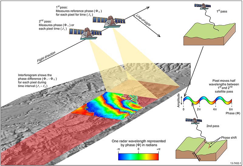
Fig. 7 InSAR schematic depicting how phase shifts can result from earthquake displacements. Source)
```{seealso}
- [ESA Documentation](https://sentinel.esa.int/web/sentinel/missions/sentinel-1)
- [Alaska Satellite Facility Documentation](https://asf.alaska.edu/data-sets/sar-data-sets/sentinel-1/)
Search and Discovery
Public Archives
The most common data products you’ll encounter for Sentinel-1 are GRD (just amplitude) and SLC (amplitude+phase). These are level-1 products that many higher-level scientific products are derived from.
Level-1 data is typically stored in radar coordinates. For SLCs, pixels are rectangular with a ratio of about 6:1 for range:azimuth, given the different resolutions in these orthogonal directions. You might notice ground control points (GCPs) stored in GRD and SLC metadata for approximate geocoding, but you need to use advanced processing pipelines to accurately geocode and generate higher level products such as interferograms [Yagüe-Martínez et al., 2016].
Higher-level products
There are also a growing number of cloud-hosted archives of processed Sentinel-1 data including global \(\sigma_0\) radiometric terrain corrected (RTC) in Google Earth Engine, \(\gamma_0\) RTC data as an AWS public dataset. Generating higher-level products often requires using a digital elevation model, so it’s important to be aware of the resolution and acquisition time of that digital elevation model. For example, two common free global digital elevation models for processing include:
Product |
Acquisition Date |
Coverage |
Resolution (m) |
Open Access |
|---|---|---|---|---|
2000-02-11 |
60\(^\circ\)N to 60\(^\circ\)S |
30 |
||
2019-12-01 -> |
global |
30 |
On-demand processing
SAR processing algorithms are complicated and resource intensive, so when possible it is nice to take advantages of services to generate higher level products. For example ASF has the HyP3 service which can generate RTC and Interferometric products: https://hyp3-docs.asf.alaska.edu
Amplitude
SAR Backscatter variations can be related to of melting snow [Small, 2011]. Cross-polarized Sentinel-1 backscatter variation has even been shown to relate to SWE [Lievens et al., 2019]. Let’s use the public RTC data from earlier and interpret values over grand mesa.
In order to work with a multidimensional timeseries stack of imagery we’ll construct a GDAL VRT file Based on the following organization: s3://sentinel-s1-rtc-indigo/tiles/RTC/1/[MODE]/[MGRS UTM zone]/[MGRS latitude label]/[MGRS Grid Square ID]/[YEAR]/[SATELLITE]_[DATE]_[TILE ID]_[ORBIT DIRECTION]/[ASSET], since the code takes a few minutes to run, we only run it if the vrt doesn’t already exist:
zone = 12
latLabel = 'S'
square = 'YJ'
year = '202*' #>=2020
date = '*' #all acquisitions
polarization = 'VV'
s3Path = f's3://sentinel-s1-rtc-indigo/tiles/RTC/1/IW/{zone}/{latLabel}/{square}/{year}/{date}/Gamma0_{polarization}.tif'

# Find imagery according to S3 path pattern
s3 = s3fs.S3FileSystem(anon=True)
keys = s3.glob(s3Path[5:]) #strip s3://
print(f'Located {len(keys)} images matching {s3Path}:')

vrtName = f'stack{zone}{latLabel}{square}.vrt'
if not os.path.exists(vrtName):
    with open('s3paths.txt', 'w') as f:
        for key in keys:
            f.write("/vsis3/%s\n" % key)

    cmd = f'gdalbuildvrt -overwrite -separate -input_file_list s3paths.txt {vrtName}'
    print(cmd)
    os.system(cmd)
Located 109 images matching s3://sentinel-s1-rtc-indigo/tiles/RTC/1/IW/12/S/YJ/202*/*/Gamma0_VV.tif:
# Load a time series we created a VRT with GDAL to facilitate this step
da3 = rioxarray.open_rasterio(vrtName, overview_level=3, chunks='auto')
da3; #omit output
# Need to add time coordinates to this data
datetimes = [pd.to_datetime(x[55:63]) for x in keys]

# add new coordinate to existing dimension
da = da3.assign_coords(time=('band', datetimes))
# make 'time' active coordinate instead of integer band
da = da.swap_dims({'band':'time'})
# Name the dataset (helpful for hvplot calls later on)
da.name = 'Gamma0VV'
da
<xarray.DataArray 'Gamma0VV' (time: 109, y: 344, x: 344)>
dask.array<open_rasterio-3cd1e87db3fe1b1fbbc4cf0696e89928<this-array>, shape=(109, 344, 344), dtype=float32, chunksize=(1, 344, 344), chunktype=numpy.ndarray>
Coordinates:
    band         (time) int64 1 2 3 4 5 6 7 8 ... 103 104 105 106 107 108 109
  * x            (x) float64 7.001e+05 7.004e+05 ... 8.093e+05 8.096e+05
  * y            (y) float64 4.4e+06 4.4e+06 4.399e+06 ... 4.291e+06 4.29e+06
    spatial_ref  int64 0
  * time         (time) datetime64[ns] 2020-08-31 2020-09-07 ... 2021-04-24
Attributes:
    _FillValue:    0.0
    scale_factor:  1.0
add_offset: 0.0- time: 109
- y: 344
- x: 344
- dask.array<chunksize=(1, 344, 344), meta=np.ndarray>
Array Chunk Bytes 49.20 MiB 462.25 kiB Shape (109, 344, 344) (1, 344, 344) Count 110 Tasks 109 Chunks Type float32 numpy.ndarray - band(time)int641 2 3 4 5 6 ... 105 106 107 108 109
array([ 1, 2, 3, 4, 5, 6, 7, 8, 9, 10, 11, 12, 13, 14, 15, 16, 17, 18, 19, 20, 21, 22, 23, 24, 25, 26, 27, 28, 29, 30, 31, 32, 33, 34, 35, 36, 37, 38, 39, 40, 41, 42, 43, 44, 45, 46, 47, 48, 49, 50, 51, 52, 53, 54, 55, 56, 57, 58, 59, 60, 61, 62, 63, 64, 65, 66, 67, 68, 69, 70, 71, 72, 73, 74, 75, 76, 77, 78, 79, 80, 81, 82, 83, 84, 85, 86, 87, 88, 89, 90, 91, 92, 93, 94, 95, 96, 97, 98, 99, 100, 101, 102, 103, 104, 105, 106, 107, 108, 109]) - x(x)float647.001e+05 7.004e+05 ... 8.096e+05
array([700119.593023, 700438.77907 , 700757.965116, ..., 808962.034884, 809281.22093 , 809600.406977]) - y(y)float644.4e+06 4.4e+06 ... 4.29e+06
array([4399880.406977, 4399561.22093 , 4399242.034884, ..., 4291037.965116, 4290718.77907 , 4290399.593023]) - spatial_ref()int640
- crs_wkt :
- PROJCS["WGS 84 / UTM zone 12N",GEOGCS["WGS 84",DATUM["WGS_1984",SPHEROID["WGS 84",6378137,298.257223563,AUTHORITY["EPSG","7030"]],AUTHORITY["EPSG","6326"]],PRIMEM["Greenwich",0,AUTHORITY["EPSG","8901"]],UNIT["degree",0.0174532925199433,AUTHORITY["EPSG","9122"]],AUTHORITY["EPSG","4326"]],PROJECTION["Transverse_Mercator"],PARAMETER["latitude_of_origin",0],PARAMETER["central_meridian",-111],PARAMETER["scale_factor",0.9996],PARAMETER["false_easting",500000],PARAMETER["false_northing",0],UNIT["metre",1,AUTHORITY["EPSG","9001"]],AXIS["Easting",EAST],AXIS["Northing",NORTH],AUTHORITY["EPSG","32612"]]
- semi_major_axis :
- 6378137.0
- semi_minor_axis :
- 6356752.314245179
- inverse_flattening :
- 298.257223563
- reference_ellipsoid_name :
- WGS 84
- longitude_of_prime_meridian :
- 0.0
- prime_meridian_name :
- Greenwich
- geographic_crs_name :
- WGS 84
- horizontal_datum_name :
- World Geodetic System 1984
- projected_crs_name :
- WGS 84 / UTM zone 12N
- grid_mapping_name :
- transverse_mercator
- latitude_of_projection_origin :
- 0.0
- longitude_of_central_meridian :
- -111.0
- false_easting :
- 500000.0
- false_northing :
- 0.0
- scale_factor_at_central_meridian :
- 0.9996
- spatial_ref :
- PROJCS["WGS 84 / UTM zone 12N",GEOGCS["WGS 84",DATUM["WGS_1984",SPHEROID["WGS 84",6378137,298.257223563,AUTHORITY["EPSG","7030"]],AUTHORITY["EPSG","6326"]],PRIMEM["Greenwich",0,AUTHORITY["EPSG","8901"]],UNIT["degree",0.0174532925199433,AUTHORITY["EPSG","9122"]],AUTHORITY["EPSG","4326"]],PROJECTION["Transverse_Mercator"],PARAMETER["latitude_of_origin",0],PARAMETER["central_meridian",-111],PARAMETER["scale_factor",0.9996],PARAMETER["false_easting",500000],PARAMETER["false_northing",0],UNIT["metre",1,AUTHORITY["EPSG","9001"]],AXIS["Easting",EAST],AXIS["Northing",NORTH],AUTHORITY["EPSG","32612"]]
- GeoTransform :
- 699960.0 319.1860465116279 0.0 4400040.0 0.0 -319.1860465116279
array(0)
- time(time)datetime64[ns]2020-08-31 ... 2021-04-24
array(['2020-08-31T00:00:00.000000000', '2020-09-07T00:00:00.000000000',
       '2020-09-12T00:00:00.000000000', '2020-09-19T00:00:00.000000000',
       '2020-09-24T00:00:00.000000000', '2020-10-01T00:00:00.000000000',
       '2020-10-06T00:00:00.000000000', '2020-10-13T00:00:00.000000000',
       '2020-10-18T00:00:00.000000000', '2020-10-25T00:00:00.000000000',
       '2020-10-30T00:00:00.000000000', '2020-11-06T00:00:00.000000000',
       '2020-11-11T00:00:00.000000000', '2020-11-18T00:00:00.000000000',
       '2020-11-23T00:00:00.000000000', '2020-11-30T00:00:00.000000000',
       '2020-12-05T00:00:00.000000000', '2020-12-12T00:00:00.000000000',
       '2020-12-17T00:00:00.000000000', '2020-12-24T00:00:00.000000000',
       '2020-12-29T00:00:00.000000000', '2020-01-05T00:00:00.000000000',
       '2020-01-12T00:00:00.000000000', '2020-01-17T00:00:00.000000000',
       '2020-01-24T00:00:00.000000000', '2020-01-29T00:00:00.000000000',
       '2020-02-10T00:00:00.000000000', '2020-02-22T00:00:00.000000000',
       '2020-02-29T00:00:00.000000000', '2020-03-05T00:00:00.000000000',
       '2020-03-12T00:00:00.000000000', '2020-03-17T00:00:00.000000000',
       '2020-03-29T00:00:00.000000000', '2020-04-05T00:00:00.000000000',
       '2020-04-10T00:00:00.000000000', '2020-04-17T00:00:00.000000000',
       '2020-04-22T00:00:00.000000000', '2020-04-29T00:00:00.000000000',
       '2020-05-04T00:00:00.000000000', '2020-05-11T00:00:00.000000000',
       '2020-05-16T00:00:00.000000000', '2020-05-23T00:00:00.000000000',
       '2020-05-28T00:00:00.000000000', '2020-06-09T00:00:00.000000000',
       '2020-06-16T00:00:00.000000000', '2020-06-21T00:00:00.000000000',
       '2020-06-28T00:00:00.000000000', '2020-07-10T00:00:00.000000000',
       '2020-07-15T00:00:00.000000000', '2020-07-22T00:00:00.000000000',
       '2020-07-27T00:00:00.000000000', '2020-08-03T00:00:00.000000000',
       '2020-08-08T00:00:00.000000000', '2020-08-15T00:00:00.000000000',
       '2020-08-20T00:00:00.000000000', '2020-08-27T00:00:00.000000000',
       '2020-09-01T00:00:00.000000000', '2020-09-08T00:00:00.000000000',
       '2020-09-13T00:00:00.000000000', '2020-09-20T00:00:00.000000000',
       '2020-09-25T00:00:00.000000000', '2020-10-02T00:00:00.000000000',
       '2020-10-07T00:00:00.000000000', '2020-10-14T00:00:00.000000000',
       '2020-10-19T00:00:00.000000000', '2020-10-26T00:00:00.000000000',
       '2020-10-31T00:00:00.000000000', '2020-11-07T00:00:00.000000000',
       '2020-11-12T00:00:00.000000000', '2020-11-19T00:00:00.000000000',
       '2020-11-24T00:00:00.000000000', '2020-12-01T00:00:00.000000000',
       '2020-12-06T00:00:00.000000000', '2020-12-13T00:00:00.000000000',
       '2020-12-18T00:00:00.000000000', '2020-12-25T00:00:00.000000000',
       '2020-12-30T00:00:00.000000000', '2021-01-05T00:00:00.000000000',
       '2021-01-10T00:00:00.000000000', '2021-01-17T00:00:00.000000000',
       '2021-01-22T00:00:00.000000000', '2021-01-29T00:00:00.000000000',
       '2021-02-27T00:00:00.000000000', '2021-03-06T00:00:00.000000000',
       '2021-03-11T00:00:00.000000000', '2021-03-18T00:00:00.000000000',
       '2021-03-23T00:00:00.000000000', '2021-03-30T00:00:00.000000000',
       '2021-04-04T00:00:00.000000000', '2021-04-11T00:00:00.000000000',
       '2021-04-16T00:00:00.000000000', '2021-04-23T00:00:00.000000000',
       '2021-01-06T00:00:00.000000000', '2021-01-11T00:00:00.000000000',
       '2021-01-18T00:00:00.000000000', '2021-01-23T00:00:00.000000000',
       '2021-01-30T00:00:00.000000000', '2021-02-04T00:00:00.000000000',
       '2021-02-11T00:00:00.000000000', '2021-02-23T00:00:00.000000000',
       '2021-02-28T00:00:00.000000000', '2021-03-07T00:00:00.000000000',
       '2021-03-19T00:00:00.000000000', '2021-03-24T00:00:00.000000000',
       '2021-03-31T00:00:00.000000000', '2021-04-05T00:00:00.000000000',
       '2021-04-12T00:00:00.000000000', '2021-04-17T00:00:00.000000000',
       '2021-04-24T00:00:00.000000000'], dtype='datetime64[ns]')
- _FillValue :
- 0.0
- scale_factor :
- 1.0
- add_offset :
- 0.0
#use a small bounding box over grand mesa (UTM coordinates)
xmin,xmax,ymin,ymax = [739186, 742748, 4.325443e+06, 4.327356e+06]
daT = da.sel(x=slice(xmin, xmax),
             y=slice(ymax, ymin))

# NOTE: this can take a while on slow internet connections, we're reading over 100 images!
all_points = daT.where(daT!=0).hvplot.scatter('time', groupby=[], dynspread=True, datashade=True)
mean_trend = daT.where(daT!=0, drop=True).mean(dim=['x','y']).hvplot.line(title='North Grand Mesa', color='red')
(all_points * mean_trend)
Interpretation
The background backscatter for this area of interest is approximately 0.5. A distinct dip in backscatter is observed during Spring snow melt April through May, with max backscatter in June corresponding to bare ground conditions. Decreasing backscatter amplitude from June onwards is likely due to increasing vegetation.
Phase
InSAR phase delays can be due to a number of factors including tectonic motions, atmospheric water vapor changes, and ionospheric conditions. The theory relating InSAR phase delays due to propagation in dry snow is described in a classic study by [Guneriussen et al., 2001].
A first-order approximation of Snow-Water-Equivalent from InSAR phase change from [Leinss et al., 2015] is:
Where \(\Delta\Phi\) is measured change in phase, \(\lambda_i\) is the radar wavelength and \(\theta_i\) is the incidence angle. This approximation assumes dry, homogeneous snow with a depth of less than 3 meters. Note also that phase delays are also be caused by changes in atmospheric water vapor, ionospheric conditions, and tectonic displacements, so care must be taken to isolate phase changes arising from SWE changes. Isolating these signals is complicated and more studies like SnowEx are necessary to validate satellite-based SWE extractions with in-situ sensors.
The following cell gets you started with plotting phase data generated by ASF’s on-demand InSAR processor. It takes about an hour for processing an interferogram, so we’ve done that ahead of time with the scripts in this repository https://github.com/snowex-hackweek/hyp3SAR, and data outputs here https://github.com/snowex-hackweek/tutorial-data.
%%bash

# Retrieve a copy of data files used in this tutorial from Zenodo.org:
# Re-running this cell will not re-download things if they already exist

mkdir -p /tmp/tutorial-data
cd /tmp/tutorial-data
wget -q -nc -O data.zip https://zenodo.org/record/5504396/files/sar.zip
unzip -q -n data.zip
rm data.zip
path = '/tmp/tutorial-data/sar/sentinel1/S1AA_20201030T131820_20201111T131820_VVP012_INT80_G_ueF_EBD2/S1AA_20201030T131820_20201111T131820_VVP012_INT80_G_ueF_EBD2_unw_phase.tif'
da = rioxarray.open_rasterio(path, masked=True).squeeze('band')
da.hvplot.image(x='x', y='y', aspect='equal', rasterize=True, cmap='plasma', title='2020/10/30_2020/11/11 Unwrapped Phase (radians)')
Interpretation
Single Sentinel-1 interferograms are usually dominated by atmospheric noise, so be cautious about interpretations of surface properties such as surface displacements or SWE changes. In theory, positive changes correspond to a path increases (or propagation delay). Phase changes are expected to be minimal for short durations, so it’s common to apply a DC-offset so that the image has a mean of 0, or normalize the image to a ground-control point with assumed zero phase shift.
Exercises
Plot a histogram of phase change
Convert the phase change into a map of SWE change
Process another interferogram between separate dates for the same area and average the two
Next steps
This tutorial just scratched the surface of Sentinel-1 SAR! Hopefully you’re now eager to explore more and utilize this dataset for SnowEx projects. Below are additional references and project ideas:
See also
expanded tutorial on AWS RTC public dataset
documentation for open source ISCE2 SAR processing software
Project Ideas
Explore RTC backscatter over different areas of interest and time ranges
Apply the C-Snow algorithm for SWE retrieval from cross-polarized backscatter with the AWS RTC public dataset
Process interferograms during dry-snow conditions and convert time series of phase changes due to snow accumulation. This would require looking at historical weather and other in-situ sensors
Compare Sentinel-1 and UAVSAR amplitude and phase products (different wavelengths and viewing geometries)