Depths and Snow Pit Data Package Contents
(12 minutes)
Learning Objectives:
Tools to access data.
Code snippets to extract and prep data.
# standard imports
import os
from pathlib import Path
import glob
import pandas as pd
import numpy as np

#plotting imports
import matplotlib as mpl
import matplotlib.pyplot as plt
plt.style.use(['seaborn-notebook'])
Access tutorial data from Zenodo
We’ve archived datasets used for 2021 Hackweek tutorials on Zenodo, to ensure that these tutorials can be run in the future. The following code pulls data from the Zenodo ‘record’ and unzips it:
%%bash

# Retrieve a copy of data files used in this tutorial from Zenodo.org:
# Re-running this cell will not re-download things if they already exist

mkdir -p /tmp/tutorial-data
cd /tmp/tutorial-data
wget -q -nc -O data.zip https://zenodo.org/record/5504396/files/core-datasets.zip
unzip -q -n data.zip
rm data.zip
TUTORIAL_DATA = '/tmp/tutorial-data/core-datasets'
Download snow depth data from NSIDC
From the SnowEx20 Depth Probe Landing Page, you can download data and access the User’s Guide
The Community Snow Depth Probe data package is a single CSV with over 36,000 geolocated snow depths! Three different instrument types were used to measure depths and are recorded in the Measurement Tool column.
Programmatically download snow depth data from NSIDC
#os.chmod('/home/jovyan/.netrc', 0o600) #only necessary on snowex hackweek jupyterhub
#%run './scripts/nsidc-download_SNEX20_SD.001.py'
#print('Grand Mesa 2020 Snow Depth data download complete')
#path = Path('./data/depths/')

#for filename in path.glob('*.csv'):
#    print(filename.name)
Read the Depth File
df = pd.read_csv(f'{TUTORIAL_DATA}/depths/SnowEx2020_SnowDepths_COGM_alldepths_v01.csv', sep=',', header=0, parse_dates=[[2,3]]) #parse the date[2] and time[3] columns such that they are read in as datetime dtypes

print('file has been read, and is ready to use.')
file has been read, and is ready to use.
# check data types for each column
df.dtypes
Date (yyyymmdd)_Time (hh:mm, local, MST)                           datetime64[ns]
Measurement Tool (MP = Magnaprobe; M2 = Mesa 2; PR = Pit Ruler)            object
ID                                                                          int64
PitID                                                                      object
Longitude                                                                 float64
Latitude                                                                  float64
Easting                                                                   float64
Northing                                                                  float64
Depth (cm)                                                                  int64
elevation (m)                                                             float64
equipment                                                                  object
Version Number                                                              int64
dtype: object
Prep for Data Analysis
# rename some columns for ease further down
df.rename(columns = {
    'Measurement Tool (MP = Magnaprobe; M2 = Mesa 2; PR = Pit Ruler)':'Measurement Tool',
    'Date (yyyymmdd)_Time (hh:mm, local, MST)': "Datetime"},
          inplace = True)

# set up filter for IOP date range
start = pd.to_datetime('1/28/2020') #first day of GM IOP campaign
end   = pd.to_datetime('2/12/2020') #last day of GM IOP campaign

# filter the IOP date range
df = df[(df['Datetime'] >= start) & (df['Datetime'] <= end)]

print('DataFrame shape is: ', df.shape)
df.head()
DataFrame shape is: (36388, 12)
| Datetime | Measurement Tool | ID | PitID | Longitude | Latitude | Easting | Northing | Depth (cm) | elevation (m) | equipment | Version Number | |
|---|---|---|---|---|---|---|---|---|---|---|---|---|
| 0 | 2020-01-28 11:48:00 | MP | 100000 | 8N58 | -108.13515 | 39.03045 | 747987.62 | 4324061.71 | 94 | 3148.2 | CRREL_B | 1 |
| 1 | 2020-01-28 11:48:00 | MP | 100001 | 8N58 | -108.13516 | 39.03045 | 747986.75 | 4324061.68 | 74 | 3148.3 | CRREL_B | 1 |
| 2 | 2020-01-28 11:48:00 | MP | 100002 | 8N58 | -108.13517 | 39.03045 | 747985.89 | 4324061.65 | 90 | 3148.2 | CRREL_B | 1 |
| 3 | 2020-01-28 11:48:00 | MP | 100003 | 8N58 | -108.13519 | 39.03044 | 747984.19 | 4324060.49 | 87 | 3148.6 | CRREL_B | 1 |
| 4 | 2020-01-28 11:48:00 | MP | 100004 | 8N58 | -108.13519 | 39.03042 | 747984.26 | 4324058.27 | 90 | 3150.1 | CRREL_B | 1 |
Use .groupby() to sort the data set
# group data by the measurement tool
gb = df.groupby('Measurement Tool', as_index=False).mean().round(1)

# show mean snow depth from each tool
gb[['Measurement Tool', 'Depth (cm)']]
| Measurement Tool | Depth (cm) | |
|---|---|---|
| 0 | M2 | 97.0 |
| 1 | MP | 94.8 |
| 2 | PR | 94.6 |
Your turn
# group data by the snow pit ID


# show mean snow depth around each snow pit


#(hint: what is the pit id column called? If you're not sure you can use df.columns to see a list of column names. Consider using .head() to display only the first 5 returns)
Find depths associated with a certain measurement tool
print('List of Measurement Tools: ', df['Measurement Tool'].unique())
List of Measurement Tools: ['MP' 'M2' 'PR']
r = df.loc[df['Measurement Tool'] == 'PR']
print('DataFrame shape is: ', r.shape)
r.head()
DataFrame shape is: (148, 12)
| Datetime | Measurement Tool | ID | PitID | Longitude | Latitude | Easting | Northing | Depth (cm) | elevation (m) | equipment | Version Number | |
|---|---|---|---|---|---|---|---|---|---|---|---|---|
| 37755 | 2020-01-30 11:24:00 | PR | 300001 | 7C15 | -108.19593 | 39.04563 | 742673.94 | 4325582.37 | 100 | 3048.699951 | ruler | 1 |
| 37756 | 2020-01-29 15:00:00 | PR | 300002 | 6C37 | -108.14791 | 39.00760 | 746962.00 | 4321491.00 | 117 | 3087.709961 | ruler | 1 |
| 37757 | 2020-02-09 12:30:00 | PR | 300003 | 8C31 | -108.16401 | 39.02144 | 745520.00 | 4322983.00 | 98 | 3099.639893 | ruler | 1 |
| 37758 | 2020-01-28 09:13:00 | PR | 300004 | 6N18 | -108.19103 | 39.03404 | 743137.23 | 4324309.43 | 92 | 3055.590088 | ruler | 1 |
| 37760 | 2020-02-10 10:30:00 | PR | 300006 | 8S41 | -108.14962 | 39.01659 | 746783.00 | 4322484.00 | 95 | 3113.870117 | ruler | 1 |
Your turn
# find all depths recorded by the Mesa2


# (hint: copy/paste is your friend)
Let’s make sure we all have the same pd.DataFrame() again
# pit ruler snow depths from Grand Mesa IOP
r = df.loc[df['Measurement Tool'] == 'PR']
print( 'DataFrame is back to only pit ruler depths')
DataFrame is back to only pit ruler depths
Plotting
# plot pit ruler depths
ax = r.plot(x='Easting', y='Northing', c='Depth (cm)', kind='scatter', alpha=0.7, colorbar=True, colormap='PuBu', legend=True)
ax.set_title('Grand Mesa Pit Ruler Depths')
ax.set_xlabel('Easting [m]')
ax.set_ylabel('Northing [m]')
plt.show()

print('Notice the point on the far right - that is the "GML" or Grand Mesa Lodge pit where all instruments were deployed for a comparison study. pitID=GML')
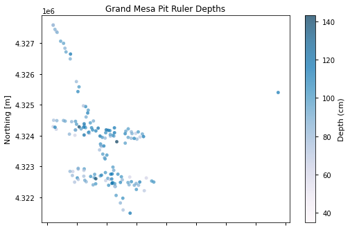
Notice the point on the far right - that is the "GML" or Grand Mesa Lodge pit where all instruments were deployed for a comparison study. pitID=GML
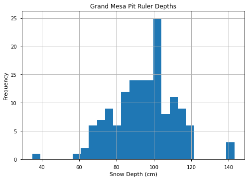
# plot histogram of pit ruler depths
ax = r['Depth (cm)'].plot.hist(bins=25)
ax.grid()
ax.set_title('Grand Mesa Pit Ruler Depths')
ax.set_xlabel('Snow Depth (cm)')
ax.set_ylabel('Frequency')
Text(0, 0.5, 'Frequency')
Download snow pit data from NSIDC
From the SnowEx20 Snow Pit Landing Page, you can download data and access the User’s Guide.
Programmatically download snow pit data from NSIDC
# load snow pit data
#%run 'scripts/nsidc-download_SNEX20_GM_SP.001.py'
#print('Grand Mesa 2020 Snow Pit data download complete')
Don’t want to work with all the files? Method to filter files
# what files would you like to find?
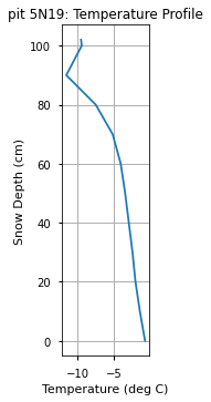
parameter = 'temperature'
pitID = '5N19'
date = '20200128'
path = '{}/pits/SnowEx20_SnowPits_GMIOP_{}_{}_{}_v01.csv'.format(TUTORIAL_DATA, date, pitID, parameter)
Read the Pit Parameter File
t = pd.read_csv(path, header=7)
t
| # Height (cm) | Temperature (deg C) | |
|---|---|---|
| 0 | 102 | -9.5 |
| 1 | 100 | -9.4 |
| 2 | 90 | -11.5 |
| 3 | 80 | -7.5 |
| 4 | 70 | -5.2 |
| 5 | 60 | -4.1 |
| 6 | 50 | -3.5 |
| 7 | 40 | -3.0 |
| 8 | 30 | -2.5 |
| 9 | 20 | -2.1 |
| 10 | 10 | -1.5 |
| 11 | 0 | -0.8 |
Plotting
# plot temperature
ax = t.plot(x='Temperature (deg C)',y='# Height (cm)', legend=False)
ax.set_aspect(0.4)
ax.grid()
ax.set_title('pit {}: Temperature Profile'.format(pitID))
ax.set_xlabel('Temperature (deg C)')
ax.set_ylabel('Snow Depth (cm)')
Text(0, 0.5, 'Snow Depth (cm)')
# grab a different pit parameter file
parameter = 'density'
path = '/tmp/tutorial-data/core-datasets/pits/SnowEx20_SnowPits_GMIOP_{}_{}_{}_v01.csv'.format(date, pitID, parameter)
d = pd.read_csv(path, header=7)
d
| # Top (cm) | Bottom (cm) | Density A (kg/m3) | Density B (kg/m3) | Density C (kg/m3) | |
|---|---|---|---|---|---|
| 0 | 102.0 | 92.0 | 136.0 | 138.0 | NaN |
| 1 | 92.0 | 82.0 | 193.0 | 192.0 | NaN |
| 2 | 82.0 | 72.0 | 232.0 | 221.0 | NaN |
| 3 | 72.0 | 62.0 | 262.0 | 260.0 | NaN |
| 4 | 62.0 | 52.0 | 275.0 | 278.0 | NaN |
| 5 | 52.0 | 42.0 | 261.0 | 252.0 | NaN |
| 6 | 42.0 | 32.0 | 267.0 | 269.0 | NaN |
| 7 | 32.0 | 22.0 | 336.0 | 367.0 | NaN |
| 8 | 22.0 | 12.0 | 268.0 | 246.0 | NaN |
| 9 | 12.0 | 2.0 | 262.0 | 271.0 | NaN |
# get the average density
d['Avg Density (kg/m3)'] = d[['Density A (kg/m3)', 'Density B (kg/m3)', 'Density C (kg/m3)']].mean(axis=1, skipna=True)
d
| # Top (cm) | Bottom (cm) | Density A (kg/m3) | Density B (kg/m3) | Density C (kg/m3) | Avg Density (kg/m3) | |
|---|---|---|---|---|---|---|
| 0 | 102.0 | 92.0 | 136.0 | 138.0 | NaN | 137.0 |
| 1 | 92.0 | 82.0 | 193.0 | 192.0 | NaN | 192.5 |
| 2 | 82.0 | 72.0 | 232.0 | 221.0 | NaN | 226.5 |
| 3 | 72.0 | 62.0 | 262.0 | 260.0 | NaN | 261.0 |
| 4 | 62.0 | 52.0 | 275.0 | 278.0 | NaN | 276.5 |
| 5 | 52.0 | 42.0 | 261.0 | 252.0 | NaN | 256.5 |
| 6 | 42.0 | 32.0 | 267.0 | 269.0 | NaN | 268.0 |
| 7 | 32.0 | 22.0 | 336.0 | 367.0 | NaN | 351.5 |
| 8 | 22.0 | 12.0 | 268.0 | 246.0 | NaN | 257.0 |
| 9 | 12.0 | 2.0 | 262.0 | 271.0 | NaN | 266.5 |
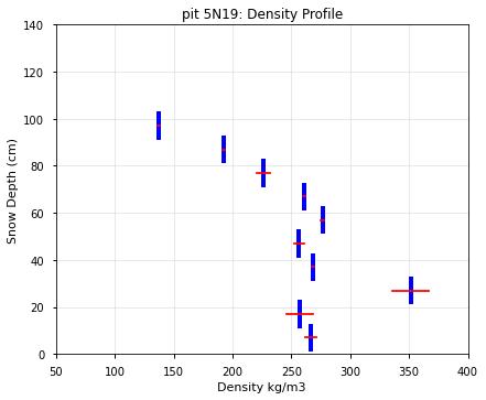
def plot_density(ax, dataframe):

    '''
    This function helps you plot density profiles from snow pits. Use it to iterate through
    DataFrame rows and plot the density for each top and bottom segment.

    '''

    for index, row in dataframe.iterrows():
        # plot blue bars to represent 10cm density intervals
        top = row['# Top (cm)']
        bottom = row['Bottom (cm)']
        dens = row["Avg Density (kg/m3)"]
        ax.plot([dens, dens],[bottom, top], color='blue', linewidth=4)

        # plot a red cross to show the spread between A and B samples
        densA = row["Density A (kg/m3)"]
        densB = row["Density B (kg/m3)"]
        middle = bottom + 5.
        ax.plot([densA, densB],[middle,middle], color='red')

    return ax

fig, ax = plt.subplots()
ax = plot_density(ax, d)
ax.set_xlim(50, 400)
ax.set_ylim(0, 140)
ax.grid(color='lightgray', alpha=.5)
ax.set_aspect(2)
ax.set_title('pit {}: Density Profile'.format(pitID))
ax.set_xlabel('Density kg/m3')
ax.set_ylabel('Snow Depth (cm)')
Text(0, 0.5, 'Snow Depth (cm)')