.ipynb .pdf

repository open issue suggest edit

Contents

Visualizing and Comparing LIS Output

LIS Output Primer

LIS writes model state variables to disk at a frequency selected by the user (e.g., 6-hourly, daily, monthly). The LIS output we will be exploring was originally generated as daily NetCDF files, meaning one NetCDF was written per simulated day. We have converted these NetCDF files into a Zarr store for improved performance in the cloud.

Import Libraries

# interface to Amazon S3 filesystem
import s3fs

# interact with n-d arrays
import numpy as np
import xarray as xr

# interact with tabular data (incl. spatial)
import pandas as pd
import geopandas as gpd

# interactive plots
import holoviews as hv
import geoviews as gv
import hvplot.pandas
import hvplot.xarray

# used to find nearest grid cell to a given location
from scipy.spatial import distance

# set bokeh as the holoviews plotting backend
hv.extension('bokeh')

Load the LIS Output

The xarray library makes working with labelled n-dimensional arrays easy and efficient. If you’re familiar with the pandas library it should feel pretty familiar.

Here we load the LIS output into an xarray.Dataset object:

# create S3 filesystem object
s3 = s3fs.S3FileSystem(anon=False)

# define the name of our S3 bucket
bucket_name = 'eis-dh-hydro/SNOWEX-HACKWEEK'

# define path to store on S3
lis_output_s3_path = f's3://{bucket_name}/DA_SNODAS/SURFACEMODEL/LIS_HIST.d01.zarr/'

# create key-value mapper for S3 object (required to read data stored on S3)
lis_output_mapper = s3.get_mapper(lis_output_s3_path)

# open the dataset
lis_output_ds = xr.open_zarr(lis_output_mapper, consolidated=True)

# drop some unneeded variables
lis_output_ds = lis_output_ds.drop_vars(['_history', '_eis_source_path'])

Explore the Data

Display an interactive widget for inspecting the dataset by running a cell containing the variable name. Expand the dropdown menus and click on the document and database icons to inspect the variables and attributes.

lis_output_ds

<xarray.Dataset>
Dimensions:           (time: 730, north_south: 215, east_west: 361, SoilMoist_profiles: 4)
Coordinates:
  * time              (time) datetime64[ns] 2016-10-01 2016-10-02 ... 2018-09-30
Dimensions without coordinates: north_south, east_west, SoilMoist_profiles
Data variables: (12/26)
    Albedo_tavg       (time, north_south, east_west) float32 dask.array<chunksize=(1, 215, 361), meta=np.ndarray>
    CanopInt_tavg     (time, north_south, east_west) float32 dask.array<chunksize=(1, 215, 361), meta=np.ndarray>
    ECanop_tavg       (time, north_south, east_west) float32 dask.array<chunksize=(1, 215, 361), meta=np.ndarray>
    ESoil_tavg        (time, north_south, east_west) float32 dask.array<chunksize=(1, 215, 361), meta=np.ndarray>
    GPP_tavg          (time, north_south, east_west) float32 dask.array<chunksize=(1, 215, 361), meta=np.ndarray>
    LAI_tavg          (time, north_south, east_west) float32 dask.array<chunksize=(1, 215, 361), meta=np.ndarray>
    ...                ...
    Swnet_tavg        (time, north_south, east_west) float32 dask.array<chunksize=(1, 215, 361), meta=np.ndarray>
    TVeg_tavg         (time, north_south, east_west) float32 dask.array<chunksize=(1, 215, 361), meta=np.ndarray>
    TWS_tavg          (time, north_south, east_west) float32 dask.array<chunksize=(1, 215, 361), meta=np.ndarray>
    TotalPrecip_tavg  (time, north_south, east_west) float32 dask.array<chunksize=(1, 215, 361), meta=np.ndarray>
    lat               (time, north_south, east_west) float32 dask.array<chunksize=(1, 215, 361), meta=np.ndarray>
    lon               (time, north_south, east_west) float32 dask.array<chunksize=(1, 215, 361), meta=np.ndarray>
Attributes: (12/14)
    DX:                      0.10000000149011612
    DY:                      0.10000000149011612
    MAP_PROJECTION:          EQUIDISTANT CYLINDRICAL
    NUM_SOIL_LAYERS:         4
    SOIL_LAYER_THICKNESSES:  [10.0, 30.000001907348633, 60.000003814697266, 1...
    SOUTH_WEST_CORNER_LAT:   28.549999237060547
    ...                      ...
    conventions:             CF-1.6
    institution:             NASA GSFC
    missing_value:           -9999.0
    references:              Kumar_etal_EMS_2006, Peters-Lidard_etal_ISSE_2007
    source:                  Noah-MP.4.0.1
    title:                   LIS land surface model output

Accessing Attributes

Dataset attributes (metadata) are accessible via the attrs attribute:

lis_output_ds.attrs

{'DX': 0.10000000149011612,
 'DY': 0.10000000149011612,
 'MAP_PROJECTION': 'EQUIDISTANT CYLINDRICAL',
 'NUM_SOIL_LAYERS': 4,
 'SOIL_LAYER_THICKNESSES': [10.0,
  30.000001907348633,
  60.000003814697266,
  100.0],
 'SOUTH_WEST_CORNER_LAT': 28.549999237060547,
 'SOUTH_WEST_CORNER_LON': -113.94999694824219,
 'comment': 'website: http://lis.gsfc.nasa.gov/',
 'conventions': 'CF-1.6',
 'institution': 'NASA GSFC',
 'missing_value': -9999.0,
 'references': 'Kumar_etal_EMS_2006, Peters-Lidard_etal_ISSE_2007',
 'source': 'Noah-MP.4.0.1',
 'title': 'LIS land surface model output'}

Accessing Variables

Variables can be accessed using either dot notation or square bracket notation:

# dot notation
lis_output_ds.SnowDepth_tavg

<xarray.DataArray 'SnowDepth_tavg' (time: 730, north_south: 215, east_west: 361)>
dask.array<open_dataset-7d66e42249419f6b85d6bd66542e643aSnowDepth_tavg, shape=(730, 215, 361), dtype=float32, chunksize=(1, 215, 361), chunktype=numpy.ndarray>
Coordinates:
  * time     (time) datetime64[ns] 2016-10-01 2016-10-02 ... 2018-09-30
Dimensions without coordinates: north_south, east_west
Attributes:
    long_name:      snow depth
    standard_name:  snow_depth
    units:          m
    vmax:           999999986991104.0
    vmin:           -999999986991104.0

# square bracket notation
lis_output_ds['SnowDepth_tavg']

<xarray.DataArray 'SnowDepth_tavg' (time: 730, north_south: 215, east_west: 361)>
dask.array<open_dataset-7d66e42249419f6b85d6bd66542e643aSnowDepth_tavg, shape=(730, 215, 361), dtype=float32, chunksize=(1, 215, 361), chunktype=numpy.ndarray>
Coordinates:
  * time     (time) datetime64[ns] 2016-10-01 2016-10-02 ... 2018-09-30
Dimensions without coordinates: north_south, east_west
Attributes:
    long_name:      snow depth
    standard_name:  snow_depth
    units:          m
    vmax:           999999986991104.0
    vmin:           -999999986991104.0

Which syntax should I use?

While both syntaxes perform the same function, the square-bracket syntax is useful when interacting with a dataset programmatically. For example, we can define a variable varname that stores the name of the variable in the dataset we want to access and then use that with the square-brackets notation:

varname = 'SnowDepth_tavg'

lis_output_ds[varname]

<xarray.DataArray 'SnowDepth_tavg' (time: 730, north_south: 215, east_west: 361)>
dask.array<open_dataset-7d66e42249419f6b85d6bd66542e643aSnowDepth_tavg, shape=(730, 215, 361), dtype=float32, chunksize=(1, 215, 361), chunktype=numpy.ndarray>
Coordinates:
  * time     (time) datetime64[ns] 2016-10-01 2016-10-02 ... 2018-09-30
Dimensions without coordinates: north_south, east_west
Attributes:
    long_name:      snow depth
    standard_name:  snow_depth
    units:          m
    vmax:           999999986991104.0
    vmin:           -999999986991104.0

The dot notation syntax will not work this way because xarray tries to find a variable in the dataset named varname instead of the value of the varname variable. When xarray can’t find this variable, it throws an error:

# uncomment and run the code below to see the error

# varname = 'SnowDepth_tavg'

# lis_output_ds.varname

Dimensions and Coordinate Variables

The dimensions and coordinate variable fields put the “labelled” in “labelled n-dimensional arrays”:

• Dimensions: labels for each dimension in the dataset (e.g., time)

• Coordinates: labels for indexing along dimensions (e.g., '2019-01-01')

We can use these labels to select, slice, and aggregate the dataset.

Selecting/Subsetting

xarray provides two methods for selecting or subsetting along coordinate variables:

• index selection: ds.isel(time=0)

• value selection ds.sel(time='2019-01-01')

For example, we can select the first timestep from our dataset using index selection by passing the dimension name as a keyword argument:

# remember: python indexes start at 0
lis_output_ds.isel(time=0)

<xarray.Dataset>
Dimensions:           (north_south: 215, east_west: 361, SoilMoist_profiles: 4)
Coordinates:
    time              datetime64[ns] 2016-10-01
Dimensions without coordinates: north_south, east_west, SoilMoist_profiles
Data variables: (12/26)
    Albedo_tavg       (north_south, east_west) float32 dask.array<chunksize=(215, 361), meta=np.ndarray>
    CanopInt_tavg     (north_south, east_west) float32 dask.array<chunksize=(215, 361), meta=np.ndarray>
    ECanop_tavg       (north_south, east_west) float32 dask.array<chunksize=(215, 361), meta=np.ndarray>
    ESoil_tavg        (north_south, east_west) float32 dask.array<chunksize=(215, 361), meta=np.ndarray>
    GPP_tavg          (north_south, east_west) float32 dask.array<chunksize=(215, 361), meta=np.ndarray>
    LAI_tavg          (north_south, east_west) float32 dask.array<chunksize=(215, 361), meta=np.ndarray>
    ...                ...
    Swnet_tavg        (north_south, east_west) float32 dask.array<chunksize=(215, 361), meta=np.ndarray>
    TVeg_tavg         (north_south, east_west) float32 dask.array<chunksize=(215, 361), meta=np.ndarray>
    TWS_tavg          (north_south, east_west) float32 dask.array<chunksize=(215, 361), meta=np.ndarray>
    TotalPrecip_tavg  (north_south, east_west) float32 dask.array<chunksize=(215, 361), meta=np.ndarray>
    lat               (north_south, east_west) float32 dask.array<chunksize=(215, 361), meta=np.ndarray>
    lon               (north_south, east_west) float32 dask.array<chunksize=(215, 361), meta=np.ndarray>
Attributes: (12/14)
    DX:                      0.10000000149011612
    DY:                      0.10000000149011612
    MAP_PROJECTION:          EQUIDISTANT CYLINDRICAL
    NUM_SOIL_LAYERS:         4
    SOIL_LAYER_THICKNESSES:  [10.0, 30.000001907348633, 60.000003814697266, 1...
    SOUTH_WEST_CORNER_LAT:   28.549999237060547
    ...                      ...
    conventions:             CF-1.6
    institution:             NASA GSFC
    missing_value:           -9999.0
    references:              Kumar_etal_EMS_2006, Peters-Lidard_etal_ISSE_2007
    source:                  Noah-MP.4.0.1
    title:                   LIS land surface model output

Or we can use value selection to select based on the coordinate(s) (think “labels”) of a given dimension:

lis_output_ds.sel(time='2018-01-01')

<xarray.Dataset>
Dimensions:           (north_south: 215, east_west: 361, SoilMoist_profiles: 4)
Coordinates:
    time              datetime64[ns] 2018-01-01
Dimensions without coordinates: north_south, east_west, SoilMoist_profiles
Data variables: (12/26)
    Albedo_tavg       (north_south, east_west) float32 dask.array<chunksize=(215, 361), meta=np.ndarray>
    CanopInt_tavg     (north_south, east_west) float32 dask.array<chunksize=(215, 361), meta=np.ndarray>
    ECanop_tavg       (north_south, east_west) float32 dask.array<chunksize=(215, 361), meta=np.ndarray>
    ESoil_tavg        (north_south, east_west) float32 dask.array<chunksize=(215, 361), meta=np.ndarray>
    GPP_tavg          (north_south, east_west) float32 dask.array<chunksize=(215, 361), meta=np.ndarray>
    LAI_tavg          (north_south, east_west) float32 dask.array<chunksize=(215, 361), meta=np.ndarray>
    ...                ...
    Swnet_tavg        (north_south, east_west) float32 dask.array<chunksize=(215, 361), meta=np.ndarray>
    TVeg_tavg         (north_south, east_west) float32 dask.array<chunksize=(215, 361), meta=np.ndarray>
    TWS_tavg          (north_south, east_west) float32 dask.array<chunksize=(215, 361), meta=np.ndarray>
    TotalPrecip_tavg  (north_south, east_west) float32 dask.array<chunksize=(215, 361), meta=np.ndarray>
    lat               (north_south, east_west) float32 dask.array<chunksize=(215, 361), meta=np.ndarray>
    lon               (north_south, east_west) float32 dask.array<chunksize=(215, 361), meta=np.ndarray>
Attributes: (12/14)
    DX:                      0.10000000149011612
    DY:                      0.10000000149011612
    MAP_PROJECTION:          EQUIDISTANT CYLINDRICAL
    NUM_SOIL_LAYERS:         4
    SOIL_LAYER_THICKNESSES:  [10.0, 30.000001907348633, 60.000003814697266, 1...
    SOUTH_WEST_CORNER_LAT:   28.549999237060547
    ...                      ...
    conventions:             CF-1.6
    institution:             NASA GSFC
    missing_value:           -9999.0
    references:              Kumar_etal_EMS_2006, Peters-Lidard_etal_ISSE_2007
    source:                  Noah-MP.4.0.1
    title:                   LIS land surface model output

The .sel() approach also allows the use of shortcuts in some cases. For example, here we select all timesteps in the month of January 2018:

lis_output_ds.sel(time='2018-01')

<xarray.Dataset>
Dimensions:           (time: 31, north_south: 215, east_west: 361, SoilMoist_profiles: 4)
Coordinates:
  * time              (time) datetime64[ns] 2018-01-01 2018-01-02 ... 2018-01-31
Dimensions without coordinates: north_south, east_west, SoilMoist_profiles
Data variables: (12/26)
    Albedo_tavg       (time, north_south, east_west) float32 dask.array<chunksize=(1, 215, 361), meta=np.ndarray>
    CanopInt_tavg     (time, north_south, east_west) float32 dask.array<chunksize=(1, 215, 361), meta=np.ndarray>
    ECanop_tavg       (time, north_south, east_west) float32 dask.array<chunksize=(1, 215, 361), meta=np.ndarray>
    ESoil_tavg        (time, north_south, east_west) float32 dask.array<chunksize=(1, 215, 361), meta=np.ndarray>
    GPP_tavg          (time, north_south, east_west) float32 dask.array<chunksize=(1, 215, 361), meta=np.ndarray>
    LAI_tavg          (time, north_south, east_west) float32 dask.array<chunksize=(1, 215, 361), meta=np.ndarray>
    ...                ...
    Swnet_tavg        (time, north_south, east_west) float32 dask.array<chunksize=(1, 215, 361), meta=np.ndarray>
    TVeg_tavg         (time, north_south, east_west) float32 dask.array<chunksize=(1, 215, 361), meta=np.ndarray>
    TWS_tavg          (time, north_south, east_west) float32 dask.array<chunksize=(1, 215, 361), meta=np.ndarray>
    TotalPrecip_tavg  (time, north_south, east_west) float32 dask.array<chunksize=(1, 215, 361), meta=np.ndarray>
    lat               (time, north_south, east_west) float32 dask.array<chunksize=(1, 215, 361), meta=np.ndarray>
    lon               (time, north_south, east_west) float32 dask.array<chunksize=(1, 215, 361), meta=np.ndarray>
Attributes: (12/14)
    DX:                      0.10000000149011612
    DY:                      0.10000000149011612
    MAP_PROJECTION:          EQUIDISTANT CYLINDRICAL
    NUM_SOIL_LAYERS:         4
    SOIL_LAYER_THICKNESSES:  [10.0, 30.000001907348633, 60.000003814697266, 1...
    SOUTH_WEST_CORNER_LAT:   28.549999237060547
    ...                      ...
    conventions:             CF-1.6
    institution:             NASA GSFC
    missing_value:           -9999.0
    references:              Kumar_etal_EMS_2006, Peters-Lidard_etal_ISSE_2007
    source:                  Noah-MP.4.0.1
    title:                   LIS land surface model output

Select a custom range of dates using Python’s built-in slice() method:

lis_output_ds.sel(time=slice('2018-01-01', '2018-01-15'))

<xarray.Dataset>
Dimensions:           (time: 15, north_south: 215, east_west: 361, SoilMoist_profiles: 4)
Coordinates:
  * time              (time) datetime64[ns] 2018-01-01 2018-01-02 ... 2018-01-15
Dimensions without coordinates: north_south, east_west, SoilMoist_profiles
Data variables: (12/26)
    Albedo_tavg       (time, north_south, east_west) float32 dask.array<chunksize=(1, 215, 361), meta=np.ndarray>
    CanopInt_tavg     (time, north_south, east_west) float32 dask.array<chunksize=(1, 215, 361), meta=np.ndarray>
    ECanop_tavg       (time, north_south, east_west) float32 dask.array<chunksize=(1, 215, 361), meta=np.ndarray>
    ESoil_tavg        (time, north_south, east_west) float32 dask.array<chunksize=(1, 215, 361), meta=np.ndarray>
    GPP_tavg          (time, north_south, east_west) float32 dask.array<chunksize=(1, 215, 361), meta=np.ndarray>
    LAI_tavg          (time, north_south, east_west) float32 dask.array<chunksize=(1, 215, 361), meta=np.ndarray>
    ...                ...
    Swnet_tavg        (time, north_south, east_west) float32 dask.array<chunksize=(1, 215, 361), meta=np.ndarray>
    TVeg_tavg         (time, north_south, east_west) float32 dask.array<chunksize=(1, 215, 361), meta=np.ndarray>
    TWS_tavg          (time, north_south, east_west) float32 dask.array<chunksize=(1, 215, 361), meta=np.ndarray>
    TotalPrecip_tavg  (time, north_south, east_west) float32 dask.array<chunksize=(1, 215, 361), meta=np.ndarray>
    lat               (time, north_south, east_west) float32 dask.array<chunksize=(1, 215, 361), meta=np.ndarray>
    lon               (time, north_south, east_west) float32 dask.array<chunksize=(1, 215, 361), meta=np.ndarray>
Attributes: (12/14)
    DX:                      0.10000000149011612
    DY:                      0.10000000149011612
    MAP_PROJECTION:          EQUIDISTANT CYLINDRICAL
    NUM_SOIL_LAYERS:         4
    SOIL_LAYER_THICKNESSES:  [10.0, 30.000001907348633, 60.000003814697266, 1...
    SOUTH_WEST_CORNER_LAT:   28.549999237060547
    ...                      ...
    conventions:             CF-1.6
    institution:             NASA GSFC
    missing_value:           -9999.0
    references:              Kumar_etal_EMS_2006, Peters-Lidard_etal_ISSE_2007
    source:                  Noah-MP.4.0.1
    title:                   LIS land surface model output

Latitude and Longitude

You may have noticed that latitude (lat) and longitude (lon) are listed as data variables, not coordinate variables. This dataset would be easier to work with if lat and lon were coordinate variables and dimensions. Here we define a helper function that reads the spatial information from the dataset attributes, generates arrays containing the lat and lon values, and appends them to the dataset:

def add_latlon_coords(dataset: xr.Dataset)->xr.Dataset:
    """Adds lat/lon as dimensions and coordinates to an xarray.Dataset object."""
    
    # get attributes from dataset
    attrs = dataset.attrs
    
    # get x, y resolutions
    dx = round(float(attrs['DX']), 3)
    dy = round(float(attrs['DY']), 3)
    
    # get grid cells in x, y dimensions
    ew_len = len(dataset['east_west'])
    ns_len = len(dataset['north_south'])
    
    # get lower-left lat and lon
    ll_lat = round(float(attrs['SOUTH_WEST_CORNER_LAT']), 3)
    ll_lon = round(float(attrs['SOUTH_WEST_CORNER_LON']), 3)
    
    # calculate upper-right lat and lon
    ur_lat =  ll_lat + (dy * ns_len)
    ur_lon = ll_lon + (dx * ew_len)
    
    # define the new coordinates
    coords = {
        # create an arrays containing the lat/lon at each gridcell
        'lat': np.linspace(ll_lat, ur_lat, ns_len, dtype=np.float32, endpoint=False),
        'lon': np.linspace(ll_lon, ur_lon, ew_len, dtype=np.float32, endpoint=False)
    }
    
    lon_attrs = dataset.lon.attrs
    lat_attrs = dataset.lat.attrs
    
    # rename the original lat and lon variables
    dataset = dataset.rename({'lon':'orig_lon', 'lat':'orig_lat'})
    # rename the grid dimensions to lat and lon
    dataset = dataset.rename({'north_south': 'lat', 'east_west': 'lon'})
    # assign the coords above as coordinates
    dataset = dataset.assign_coords(coords)
    dataset.lon.attrs = lon_attrs
    dataset.lat.attrs = lat_attrs
    
    return dataset

Now that the function is defined, let’s use it to append lat and lon coordinates to the LIS output:

lis_output_ds = add_latlon_coords(lis_output_ds)

Inspect the dataset:

lis_output_ds

<xarray.Dataset>
Dimensions:           (time: 730, lat: 215, lon: 361, SoilMoist_profiles: 4)
Coordinates:
  * time              (time) datetime64[ns] 2016-10-01 2016-10-02 ... 2018-09-30
  * lat               (lat) float32 28.55 28.65 28.75 ... 49.75 49.85 49.95
  * lon               (lon) float32 -113.9 -113.8 -113.8 ... -78.05 -77.95
Dimensions without coordinates: SoilMoist_profiles
Data variables: (12/26)
    Albedo_tavg       (time, lat, lon) float32 dask.array<chunksize=(1, 215, 361), meta=np.ndarray>
    CanopInt_tavg     (time, lat, lon) float32 dask.array<chunksize=(1, 215, 361), meta=np.ndarray>
    ECanop_tavg       (time, lat, lon) float32 dask.array<chunksize=(1, 215, 361), meta=np.ndarray>
    ESoil_tavg        (time, lat, lon) float32 dask.array<chunksize=(1, 215, 361), meta=np.ndarray>
    GPP_tavg          (time, lat, lon) float32 dask.array<chunksize=(1, 215, 361), meta=np.ndarray>
    LAI_tavg          (time, lat, lon) float32 dask.array<chunksize=(1, 215, 361), meta=np.ndarray>
    ...                ...
    Swnet_tavg        (time, lat, lon) float32 dask.array<chunksize=(1, 215, 361), meta=np.ndarray>
    TVeg_tavg         (time, lat, lon) float32 dask.array<chunksize=(1, 215, 361), meta=np.ndarray>
    TWS_tavg          (time, lat, lon) float32 dask.array<chunksize=(1, 215, 361), meta=np.ndarray>
    TotalPrecip_tavg  (time, lat, lon) float32 dask.array<chunksize=(1, 215, 361), meta=np.ndarray>
    orig_lat          (time, lat, lon) float32 dask.array<chunksize=(1, 215, 361), meta=np.ndarray>
    orig_lon          (time, lat, lon) float32 dask.array<chunksize=(1, 215, 361), meta=np.ndarray>
Attributes: (12/14)
    DX:                      0.10000000149011612
    DY:                      0.10000000149011612
    MAP_PROJECTION:          EQUIDISTANT CYLINDRICAL
    NUM_SOIL_LAYERS:         4
    SOIL_LAYER_THICKNESSES:  [10.0, 30.000001907348633, 60.000003814697266, 1...
    SOUTH_WEST_CORNER_LAT:   28.549999237060547
    ...                      ...
    conventions:             CF-1.6
    institution:             NASA GSFC
    missing_value:           -9999.0
    references:              Kumar_etal_EMS_2006, Peters-Lidard_etal_ISSE_2007
    source:                  Noah-MP.4.0.1
    title:                   LIS land surface model output

Now lat and lon are listed as coordinate variables and have replaced the north_south and east_west dimensions. This will make it easier to spatially subset the dataset!

Basic Spatial Subsetting

We can use the slice() function we used above on the lat and lon dimensions to select data between a range of latitudes and longitudes:

lis_output_ds.sel(lat=slice(37, 41), lon=slice(-110, -101))

<xarray.Dataset>
Dimensions:           (time: 730, lat: 40, lon: 90, SoilMoist_profiles: 4)
Coordinates:
  * time              (time) datetime64[ns] 2016-10-01 2016-10-02 ... 2018-09-30
  * lat               (lat) float32 37.05 37.15 37.25 ... 40.75 40.85 40.95
  * lon               (lon) float32 -109.9 -109.8 -109.8 ... -101.2 -101.1
Dimensions without coordinates: SoilMoist_profiles
Data variables: (12/26)
    Albedo_tavg       (time, lat, lon) float32 dask.array<chunksize=(1, 40, 90), meta=np.ndarray>
    CanopInt_tavg     (time, lat, lon) float32 dask.array<chunksize=(1, 40, 90), meta=np.ndarray>
    ECanop_tavg       (time, lat, lon) float32 dask.array<chunksize=(1, 40, 90), meta=np.ndarray>
    ESoil_tavg        (time, lat, lon) float32 dask.array<chunksize=(1, 40, 90), meta=np.ndarray>
    GPP_tavg          (time, lat, lon) float32 dask.array<chunksize=(1, 40, 90), meta=np.ndarray>
    LAI_tavg          (time, lat, lon) float32 dask.array<chunksize=(1, 40, 90), meta=np.ndarray>
    ...                ...
    Swnet_tavg        (time, lat, lon) float32 dask.array<chunksize=(1, 40, 90), meta=np.ndarray>
    TVeg_tavg         (time, lat, lon) float32 dask.array<chunksize=(1, 40, 90), meta=np.ndarray>
    TWS_tavg          (time, lat, lon) float32 dask.array<chunksize=(1, 40, 90), meta=np.ndarray>
    TotalPrecip_tavg  (time, lat, lon) float32 dask.array<chunksize=(1, 40, 90), meta=np.ndarray>
    orig_lat          (time, lat, lon) float32 dask.array<chunksize=(1, 40, 90), meta=np.ndarray>
    orig_lon          (time, lat, lon) float32 dask.array<chunksize=(1, 40, 90), meta=np.ndarray>
Attributes: (12/14)
    DX:                      0.10000000149011612
    DY:                      0.10000000149011612
    MAP_PROJECTION:          EQUIDISTANT CYLINDRICAL
    NUM_SOIL_LAYERS:         4
    SOIL_LAYER_THICKNESSES:  [10.0, 30.000001907348633, 60.000003814697266, 1...
    SOUTH_WEST_CORNER_LAT:   28.549999237060547
    ...                      ...
    conventions:             CF-1.6
    institution:             NASA GSFC
    missing_value:           -9999.0
    references:              Kumar_etal_EMS_2006, Peters-Lidard_etal_ISSE_2007
    source:                  Noah-MP.4.0.1
    title:                   LIS land surface model output

Notice how the sizes of the lat and lon dimensions have decreased.

Subset Across Multiple Dimensions

Select snow depth for Jan 2017 within a range of lat/lon:

# define a range of dates to select
wy_2018_slice = slice('2017-10-01', '2018-09-30')
lat_slice = slice(37, 41)
lon_slice = slice(-109, -102)

# select the snow depth and subset to wy_2018_slice
snd_CO_wy2018_ds = lis_output_ds['SnowDepth_tavg'].sel(time=wy_2018_slice, lat=lat_slice, lon=lon_slice)

# inspect resulting dataset
snd_CO_wy2018_ds

<xarray.DataArray 'SnowDepth_tavg' (time: 365, lat: 40, lon: 70)>
dask.array<getitem, shape=(365, 40, 70), dtype=float32, chunksize=(1, 40, 70), chunktype=numpy.ndarray>
Coordinates:
  * time     (time) datetime64[ns] 2017-10-01 2017-10-02 ... 2018-09-30
  * lat      (lat) float32 37.05 37.15 37.25 37.35 ... 40.65 40.75 40.85 40.95
  * lon      (lon) float32 -108.9 -108.8 -108.8 -108.7 ... -102.2 -102.2 -102.1
Attributes:
    long_name:      snow depth
    standard_name:  snow_depth
    units:          m
    vmax:           999999986991104.0
    vmin:           -999999986991104.0

Plotting

We’ve imported two plotting libraries:

• matplotlib: static plots

• hvplot: interactive plots

We can make a quick matplotlib-based plot for the subsetted data using the .plot() function supplied by xarray.Dataset objects. For this example, we’ll select one day and plot it:

# simple matplotlilb plot
snd_CO_wy2018_ds.sel(time='2018-01-01').plot()

<matplotlib.collections.QuadMesh at 0x7f14d27015e0>

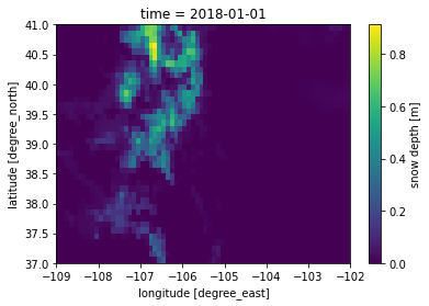
Similarly we can make an interactive plot using the hvplot accessor and specifying a quadmesh plot type:

# hvplot based map
snd_CO_20180101_plot = snd_CO_wy2018_ds.sel(time='2018-01-01').hvplot.quadmesh(geo=True, rasterize=True, project=True,
                                                                               xlabel='lon', ylabel='lat', cmap='viridis',
                                                                               tiles='EsriImagery')

snd_CO_20180101_plot

Pan, zoom, and scroll around the map. Hover over the LIS data to see the data values.

If we try to plot more than one time-step hvplot will also provide a time-slider we can use to scrub back and forth in time:

snd_CO_wy2018_ds.sel(time='2018-01').hvplot.quadmesh(geo=True, rasterize=True, project=True,
                             xlabel='lon', ylabel='lat', cmap='viridis',
                             tiles='EsriImagery')

From here on out we will stick with hvplot for plotting.

Timeseries Plots

We can generate a timeseries for a given grid cell by selecting and calling the plot function:

# define point to take timeseries (note: must be present in coordinates of dataset)
ts_lon, ts_lat = (-105.65, 40.35)

# plot timeseries (hvplot knows how to plot based on dataset's dimensionality!)
snd_CO_wy2018_ds.sel(lat=ts_lat, lon=ts_lon).hvplot(title=f'Snow Depth Timeseries @ Lon: {ts_lon}, Lat: {ts_lat}',
                                                   xlabel='Date', ylabel='Snow Depth (m)') + \
    snd_CO_20180101_plot * gv.Points([(ts_lon, ts_lat)]).opts(size=10, color='red')
    

In the next section we’ll learn how to create a timeseries over a broader area.

Aggregation

We can perform aggregation operations on the dataset such as min(), max(), mean(), and sum() by specifying the dimensions along which to perform the calculation.

For example we can calculate the mean and maximum snow depth at each grid cell over water year 2018 as follows:

# calculate the mean at each grid cell over the time dimension
mean_snd_CO_wy2018_ds = snd_CO_wy2018_ds.mean(dim='time')
max_snd_CO_wy2018_ds = snd_CO_wy2018_ds.max(dim='time')

# plot the mean and max snow depth
mean_snd_CO_wy2018_ds.hvplot.quadmesh(geo=True, rasterize=True, project=True,
                                   xlabel='lon', ylabel='lat', cmap='viridis',
                                   tiles='EsriImagery', title='Mean Snow Depth - WY2018') + \
    max_snd_CO_wy2018_ds.hvplot.quadmesh(geo=True, rasterize=True, project=True,
                                   xlabel='lon', ylabel='lat', cmap='viridis',
                                   tiles='EsriImagery', title='Max Snow Depth - WY2018')

Area Average

# take area-averaged mean at each timestep
mean_snd_CO_wy2018_ds = snd_CO_wy2018_ds.mean(['lat', 'lon'])

# inspect the dataset
mean_snd_CO_wy2018_ds

<xarray.DataArray 'SnowDepth_tavg' (time: 365)>
dask.array<mean_agg-aggregate, shape=(365,), dtype=float32, chunksize=(1,), chunktype=numpy.ndarray>
Coordinates:
  * time     (time) datetime64[ns] 2017-10-01 2017-10-02 ... 2018-09-30

# plot timeseries (hvplot knows how to plot based on dataset's dimensionality!)
mean_snd_CO_wy2018_ds.hvplot(title='Mean LIS Snow Depth for Colorado', xlabel='Date', ylabel='Snow Depth (m)')

Comparing LIS Output

Now that we’re familiar with the LIS output, let’s compare it to two other datasets: SNODAS (raster) and SNOTEL (point).

LIS (raster) vs. SNODAS (raster)

First, we’ll load the SNODAS dataset which we also have hosted on S3 as a Zarr store:

# load SNODAS dataset

#snodas depth
key = "SNODAS/snodas_snowdepth_20161001_20200930.zarr"    
snodas_depth_ds = xr.open_zarr(s3.get_mapper(f"{bucket_name}/{key}"), consolidated=True)

# apply scale factor to convert to meters (0.001 per SNODAS user guide)
snodas_depth_ds = snodas_depth_ds * 0.001

Next we define a helper function to extract the (lon, lat) of the nearest grid cell to a given point:

def nearest_grid(ds, pt):
    
    """
    Returns the nearest lon and lat to pt in a given Dataset (ds).
    
    pt : input point, tuple (longitude, latitude)
    output:
        lon, lat
    """
    
    if all(coord in list(ds.coords) for coord in ['lat', 'lon']):
        df_loc = ds[['lon', 'lat']].to_dataframe().reset_index()
    else:
        df_loc = ds[['orig_lon', 'orig_lat']].isel(time=0).to_dataframe().reset_index()
    
    loc_valid = df_loc.dropna()
    pts = loc_valid[['lon', 'lat']].to_numpy()
    idx = distance.cdist([pt], pts).argmin()
    
    return loc_valid['lon'].iloc[idx], loc_valid['lat'].iloc[idx]

The next cell will look pretty similar to what we did earlier to plot a timeseries of a single point in the LIS data. The general steps are:

• Extract the coordinates of the SNODAS grid cell nearest to our LIS grid cell (ts_lon and ts_lat from earlier)

• Subset the SNODAS and LIS data to the grid cells and date ranges of interest

• Create the plots!

# get lon, lat of snodas grid cell nearest to the LIS coordinates we used earlier
snodas_ts_lon, snodas_ts_lat = nearest_grid(snodas_depth_ds, (ts_lon, ts_lat))

# define a date range to plot (shorter = quicker for demo)
start_date, end_date = ('2018-01-01', '2018-03-01')
plot_daterange = slice(start_date, end_date)

# select SNODAS grid cell and subset to plot_daterange
snodas_snd_subset_ds = snodas_depth_ds.sel(lon=snodas_ts_lon,
                                             lat=snodas_ts_lat,
                                             time=plot_daterange)

# select LIS grid cell and subset to plot_daterange
lis_snd_subset_ds = lis_output_ds['SnowDepth_tavg'].sel(lat=ts_lat,
                                                        lon=ts_lon,
                                                        time=plot_daterange)

# create SNODAS snow depth plot
snodas_snd_plot = snodas_snd_subset_ds.hvplot(label='SNODAS')

# create LIS snow depth plot
lis_snd_plot = lis_snd_subset_ds.hvplot(label='LIS')

# create SNODAS vs LIS snow depth plot
lis_vs_snodas_snd_plot = (lis_snd_plot * snodas_snd_plot)

# display the plot
lis_vs_snodas_snd_plot.opts(title=f'Snow Depth @ Lon: {ts_lon}, Lat: {ts_lat}',
                            legend_position='right',
                            xlabel='Date',
                            ylabel='Snow Depth (m)')

LIS (raster) vs. SNODAS (raster) vs. SNOTEL (point)

Now let’s add SNOTEL point data to our plot.

First, we’re going to define some helper functions to load the SNOTEL data:

# load csv containing metadata for SNOTEL sites in a given state (e.g,. 'colorado')
def load_site(state):
    
    # define the path to the file
    key = f"SNOTEL/snotel_{state}.csv"
    
    # load the csv into a pandas DataFrame
    df = pd.read_csv(s3.open(f's3://{bucket_name}/{key}', mode='r'))
    
    return df

# load SNOTEL data for a specific site
def load_snotel_txt(state, var):
    
    # define the path to the file
    key = f"SNOTEL/snotel_{state}{var}_20162020.txt"
    
    # determine how many lines to skip in the file (they start with #)
    fh = s3.open(f"{bucket_name}/{key}")
    lines = fh.readlines()
    skips = sum(1 for ln in lines if ln.decode('ascii').startswith('#'))
    
    # load the data into a pandas DataFrame
    df = pd.read_csv(s3.open(f"s3://{bucket_name}/{key}"), skiprows=skips)
    
    # convert the Date column from strings to datetime objects
    df['Date'] = pd.to_datetime(df['Date'])
    return df

For the purposes of this tutorial let’s load the SNOTEL data for sites in Colorado. We’ll pick one site to plot in a few cells.

# load SNOTEL snow depth for Colorado into a dictionary
snotel_depth = {'CO': load_snotel_txt('CO', 'depth')}

We’ll need another helper function to load the depth data:

# get snotel depth
def get_depth(state, site, start_date, end_date):
    
    # grab the depth for the given state (e.g., CO)
    df = snotel_depth[state]
    
    # define a date range mask
    mask = (df['Date'] >= start_date) & (df['Date'] <= end_date)
    
    # use mask to subset between time range
    df = df.loc[mask]
    
    # extract timeseries for the given site
    return pd.concat([df.Date, df.filter(like=site)], axis=1).set_index('Date')

Load the site metadata for Colorado:

co_sites = load_site('colorado')

# peek at the first 5 rows
co_sites.head()

	ntwk	state	site_name	ts	lat	lon	elev
0	SNTL	CO	Apishapa (303)	NaN	37.33	-105.07	10000
1	SNTL	CO	Arapaho Ridge (1030)	NaN	40.35	-106.35	10960
2	SNTL	CO	Bear Lake (322)	NaN	40.31	-105.65	9500
3	SNTL	CO	Bear River (1061)	NaN	40.06	-107.01	9080
4	SNTL	CO	Beartown (327)	NaN	37.71	-107.51	11600

The point we’ve been using so far in the tutorial actually corresponds to the coordinates for the Bear Lake SNOTEL site along the Front Range! Let’s extract the site data for that point:

# get the depth data by passing the site name to the get_depth() function
bear_lake_snd_df = get_depth('CO', 'Bear Lake (322)', start_date, end_date)

# convert from cm to m
bear_lake_snd_df = bear_lake_snd_df / 100

Now we’re ready to plot:

# create SNOTEL plot
bear_lake_plot = bear_lake_snd_df.hvplot(label='SNOTEL')

# combine the SNOTEl plot with the LIS vs SNODAS plot
(bear_lake_plot * lis_vs_snodas_snd_plot).opts(title=f'Snow Depth @ Lon: {ts_lon}, Lat: {ts_lat}', legend_position='right')

Conclusion

You should now be more familiar with LIS data and how to interact with it in Python. The code in this notebook is a great jumping off point for developing more advanced comparisons and interactive widgets. For an example of what is possible, open the next notebook and run all the cells (Run > Run All Cells). After a few minutes, two interactive widgets will appear that allow you to explore and compare LIS output with SNODAS and SNOTEL data.

The Python code can be adapted to other LIS simulations and to other model output as well, with minor modifications. Anyone interested in testing your new skills can combine what you learned here with the other SnowEx Hackweek tutorials - try comparing the LIS output with other snow observations collected during the 2017 field campaign!

previous

NASA Land Information System (LIS)

next

Interactive Data Exploration