Time-lapse Cameras and Snow Applications
Learning Objectives
At the conclusion of this tutorial, you will…:
Know about all the time-lapse images available from the SnowEx 2017 and 2020 field campaigns
View example time-lapse images from SnowEx 2020 and visualize their locations
Access snow depth measurements extracted from the SnowEx 2020 time-lapse images
Compare snow depths from different SnowEx 2020 time-lapse cameras
Time-lapse Cameras on Grand Mesa during SnowEx Field Campaigns
Time-lapse cameras were installed in both the SnowEx 2017 and 2020 field campaigns on Grand Mesa in similar locations.
SnowEx 2017 Time-lapse Cameras
28 Total Time-lapse Cameras
Capturing the entire winter season (September 2016-June 2017)
Taking 4 photos/day at 8AM, 10AM, 12PM, 2PM, 4PM
An orange pole was installed in front of 15 cameras for snow depth measurements
Time-lapse images have been submitted to the NSIDC by Mark Raleigh with all the required metadata (e.g., locations, naming convention, etc.) for use.
SnowEx 2020 Time-lapse Cameras
29 Total Time-lapse Cameras
Capturing the entire winter season (September 2019-June 2020)
Taking 3 photos/day at 11AM, 12PM, 1PM or 2 photos/day at 11AM and 12PM
A red pole was installed in front of each camera for snow depth measurements.
Cameras were installed on the east and west side of the Grand Mesa, across a vegetation scale of 1-9, using the convention XMR:
X = East (E) or West (W) areas of the Mesa
M = number 1-9, representing 1 (least vegetation) to 9 (most vegetation). Within each vegetation class, there were three sub-classes of snow depths derived from 2017 SnowEx lidar measurements.
R = Replicate of vegetation assignment, either A, B, C, D, or E.
The complete set of time-lapse images from 2020 are in progress for submission to the NSIDC. A subset of them are available here for you to use during hackweek.
All the time-lapse camera sites from SnowEx 2017 and 2020 plotted together on Grand Mesa.
This is an interactive plot. You can zoom into the sites and click on the location icon to see the site name.
\(\color{red}{\text{2017 locations are in red}}\)
\(\color{blue}{\text{2020 locations are in blue}}\)
The following block of code to produce this plot is hidden. The interested viewer can click the … to view the Folium code.
Folium provides a simple way to visualize points, but it requires a lot of manual code to produce.
In this tutorial, we will show you how to access and view the camera data in a more automatted way. But this plot gives you an idea of where all the 2017 and 2020 sites are.
# Import the mapping package
import folium # folium interactive notebook plotting: quick start guide here: https://python-visualization.github.io/folium/quickstart.html

# Create the basemap
tooltip = "Click me!"
m = folium.Map(location=[39.035, -108.0612], tiles="Stamen Terrain", zoom_start=11, width='70%', height='70%', control_scale=True)

# Add all the points to the map
# SnowEx 2017 Sites
folium.Marker([39.0325,-108.2162], popup="TLS-A1N", tooltip=tooltip, icon=folium.Icon(color='red')).add_to(m)
folium.Marker([39.0327,-108.2152], popup="TLS-A2S", tooltip=tooltip, icon=folium.Icon(color='red')).add_to(m)
folium.Marker([39.0331,-108.2155], popup="TLS-A3E", tooltip=tooltip, icon=folium.Icon(color='red')).add_to(m)

folium.Marker([39.0098,-108.1817987], popup="TLS-D1E", tooltip=tooltip, icon=folium.Icon(color='red')).add_to(m)
folium.Marker([39.0095,-108.1812], popup="TLS-D2E", tooltip=tooltip, icon=folium.Icon(color='red')).add_to(m)
folium.Marker([39.0095,-108.1814], popup="TLS-D3W", tooltip=tooltip, icon=folium.Icon(color='red')).add_to(m)

folium.Marker([39.0081,-108.1354283], popup="TLS-F1W", tooltip=tooltip, icon=folium.Icon(color='red')).add_to(m)
folium.Marker([39.0078,-108.1364], popup="TLS-F2E", tooltip=tooltip, icon=folium.Icon(color='red')).add_to(m)
folium.Marker([39.0077,-108.1376], popup="TLS-F3N", tooltip=tooltip, icon=folium.Icon(color='red')).add_to(m)

folium.Marker([39.0328,-108.0278], popup="TLS-L1W", tooltip=tooltip, icon=folium.Icon(color='red')).add_to(m)
folium.Marker([39.0328,-108.0301], popup="TLS-L2E", tooltip=tooltip, icon=folium.Icon(color='red')).add_to(m)

folium.Marker([39.0343,-108.0554], popup="TLS-K1E", tooltip=tooltip, icon=folium.Icon(color='red')).add_to(m)
folium.Marker([39.0342,-108.0552], popup="TLS-K2E", tooltip=tooltip, icon=folium.Icon(color='red')).add_to(m)
folium.Marker([39.0342,-108.0543], popup="TLS-K3E", tooltip=tooltip, icon=folium.Icon(color='red')).add_to(m)
folium.Marker([39.0344,-108.0543], popup="TLS-K4E", tooltip=tooltip, icon=folium.Icon(color='red')).add_to(m)
folium.Marker([39.0337,-108.054],  popup="TLS-K5E", tooltip=tooltip, icon=folium.Icon(color='red')).add_to(m)
folium.Marker([39.0342,-108.0544], popup="TLS-K6E", tooltip=tooltip, icon=folium.Icon(color='red')).add_to(m)

folium.Marker([39.0513,-108.0608], popup="TLS-J1N", tooltip=tooltip, icon=folium.Icon(color='red')).add_to(m)
folium.Marker([39.052,-108.0615],  popup="TLS-J2N", tooltip=tooltip, icon=folium.Icon(color='red')).add_to(m)
folium.Marker([39.0511,-108.0614], popup="TLS-J3S", tooltip=tooltip, icon=folium.Icon(color='red')).add_to(m)
folium.Marker([39.0507,-108.0614], popup="TLS-J4N", tooltip=tooltip, icon=folium.Icon(color='red')).add_to(m)

folium.Marker([39.0543,-108.0944], popup="CG-O1S", tooltip=tooltip, icon=folium.Icon(color='red')).add_to(m)
folium.Marker([39.0543,-108.0942], popup="CG-O2E", tooltip=tooltip, icon=folium.Icon(color='red')).add_to(m)
folium.Marker([39.0545,-108.0945], popup="CG-O3N", tooltip=tooltip, icon=folium.Icon(color='red')).add_to(m)

folium.Marker([39.0284,-107.9337], popup="TLS-N1E", tooltip=tooltip, icon=folium.Icon(color='red')).add_to(m)
folium.Marker([39.0282,-107.9886], popup="TLS-N2N", tooltip=tooltip, icon=folium.Icon(color='red')).add_to(m)
folium.Marker([39.0273,-107.9338], popup="TLS-N3E", tooltip=tooltip, icon=folium.Icon(color='red')).add_to(m)
folium.Marker([39.0271,-107.9337], popup="TLS-N4W", tooltip=tooltip, icon=folium.Icon(color='red')).add_to(m)

# SnowEx 2020 Sites
folium.Marker([39.097329,-107.887477], popup="E8A", tooltip=tooltip, icon=folium.Icon(color='blue')).add_to(m)
folium.Marker([39.097464,-107.862476], popup="E6A", tooltip=tooltip, icon=folium.Icon(color='blue')).add_to(m)
folium.Marker([39.108011,-107.881267], popup="E3A", tooltip=tooltip, icon=folium.Icon(color='blue')).add_to(m)
folium.Marker([39.103561,-107.880742], popup="E9A", tooltip=tooltip, icon=folium.Icon(color='blue')).add_to(m)
folium.Marker([39.100639,-107.900614], popup="E9B", tooltip=tooltip, icon=folium.Icon(color='blue')).add_to(m)
folium.Marker([39.04897,-107.91307],   popup="E6B", tooltip=tooltip, icon=folium.Icon(color='blue')).add_to(m)
folium.Marker([39.098962,-107.893702], popup="E9C", tooltip=tooltip, icon=folium.Icon(color='blue')).add_to(m)
folium.Marker([39.074028,-107.877689], popup="E9D", tooltip=tooltip, icon=folium.Icon(color='blue')).add_to(m)
folium.Marker([39.059881,-107.876662], popup="E9E", tooltip=tooltip, icon=folium.Icon(color='blue')).add_to(m)
folium.Marker([39.047323,-107.923406], popup="E9F", tooltip=tooltip, icon=folium.Icon(color='blue')).add_to(m)
folium.Marker([39.03827,-107.935097],  popup="E9G", tooltip=tooltip, icon=folium.Icon(color='blue')).add_to(m)

folium.Marker([39.017236,-108.18488],  popup="W1A", tooltip=tooltip, icon=folium.Icon(color='blue')).add_to(m)
folium.Marker([39.013823,-108.208536], popup="W2A", tooltip=tooltip, icon=folium.Icon(color='blue')).add_to(m)
folium.Marker([39.050599,-108.051624], popup="W8A", tooltip=tooltip, icon=folium.Icon(color='blue')).add_to(m)
folium.Marker([39.036208,-108.161851], popup="W9A", tooltip=tooltip, icon=folium.Icon(color='blue')).add_to(m)
folium.Marker([39.013208,-108.186994], popup="W3A", tooltip=tooltip, icon=folium.Icon(color='blue')).add_to(m)
folium.Marker([39.017744,-108.165836], popup="W5A", tooltip=tooltip, icon=folium.Icon(color='blue')).add_to(m)
folium.Marker([39.012546,-108.185686], popup="W6A", tooltip=tooltip, icon=folium.Icon(color='blue')).add_to(m)


folium.Marker([39.008078,-108.18479],  popup="W1B", tooltip=tooltip, icon=folium.Icon(color='blue')).add_to(m)
folium.Marker([39.029174,-108.199952], popup="W2B", tooltip=tooltip, icon=folium.Icon(color='blue')).add_to(m)
folium.Marker([39.016342,-108.169688], popup="W6B", tooltip=tooltip, icon=folium.Icon(color='blue')).add_to(m)
folium.Marker([39.012393,-108.17615],  popup="W9B", tooltip=tooltip, icon=folium.Icon(color='blue')).add_to(m)

folium.Marker([39.012837,-108.174167], popup="W6C", tooltip=tooltip, icon=folium.Icon(color='blue')).add_to(m)
folium.Marker([39.012585,-108.095973], popup="W8C", tooltip=tooltip, icon=folium.Icon(color='blue')).add_to(m)
folium.Marker([39.024416,-108.171069], popup="W9C", tooltip=tooltip, icon=folium.Icon(color='blue')).add_to(m)
folium.Marker([39.036476,-108.155686], popup="W9D", tooltip=tooltip, icon=folium.Icon(color='blue')).add_to(m)
folium.Marker([39.033751,-108.160689], popup="W9E", tooltip=tooltip, icon=folium.Icon(color='blue')).add_to(m)
folium.Marker([39.031366,-108.180167], popup="W9G", tooltip=tooltip, icon=folium.Icon(color='blue')).add_to(m)

folium.Marker([39.033806,-108.053996], popup="TLSK20", tooltip=tooltip, icon=folium.Icon(color='blue')).add_to(m)

m
\(\color{red}{\text{2017 locations are in red}}\)
\(\color{blue}{\text{2020 locations are in blue}}\)
An automated way of viewing and mapping time-lapse photos
First, import all the packages we’ll need for this tutorial
# Packages to connect and download from the SnowEx database
import snowexsql.db # import SnowEx SQL library
from snowexsql.db import get_db # connection function from the snowexsql library
from snowexsql.data import PointData, SiteData # point and table classes
from snowexsql.conversions import query_to_geopandas # function to convert incoming data from database to geopandas df

# Packages for data analysis
import geopandas as gpd # geopandas library for data analysis and visualization
import pandas as pd # pandas as to read csv data and visualize tabular data
import numpy as np # numpy for data analysis

# Packages for data visualization
import matplotlib.pyplot as plt # matplotlib.pyplot for plotting images and graphs
from IPython.display import Image # used to display images inside the notebook
import seaborn as sns # a module that adds some plotting capabilities
import matplotlib as mpl # import all of matplotlib for plotting

# The following settings just set some defaults for the plots in this notebook
sns.set() # activates some of the default settings from seaborn
sns.set_style("dark", {"xtick.bottom": True, 'ytick.left': True}) # improves x and y ticks

plt.rcParams['figure.figsize']  = (10, 4) # figure size
plt.rcParams['axes.titlesize']  = 14 # title size
plt.rcParams['axes.labelsize']  = 12 # axes label size
plt.rcParams['xtick.labelsize'] = 11 # x tick label size
plt.rcParams['ytick.labelsize'] = 11 # y tick label size
plt.rcParams['legend.fontsize'] = 11 # legend size
mpl.rcParams['figure.dpi'] = 100
We will map 2020 time-lapse camera locations on the Grand Mesa with the 2020 snow pits for reference.
code credit: Micah Johnson
# Connect to the database
db_name = 'snow:hackweek@db.snowexdata.org/snowex'
engine, session = get_db(db_name)

# Grab all the point data that was that was measured with a time-lapse camera
qry = session.query(PointData)
qry = qry.filter(PointData.instrument == 'camera')

# Convert it to a geopandas df and visualize the dataframe
camera_depths = query_to_geopandas(qry, engine)
camera_depths.head()
| site_name | date | time_created | time_updated | id | site_id | doi | date_accessed | instrument | type | ... | longitude | northing | easting | elevation | utm_zone | geom | time | version_number | equipment | value | |
|---|---|---|---|---|---|---|---|---|---|---|---|---|---|---|---|---|---|---|---|---|---|
| 0 | Grand Mesa | 2019-10-11 | 2021-07-12 18:39:41.696919+00:00 | None | 4185953 | None | None | 2021-07-12 | camera | depth | ... | -108.184794 | 4.321444e+06 | 743766.479497 | None | 12 | POINT (743766.479 4321444.155) | 12:00:00-06:00 | None | camera id = W1B | -1.49900 |
| 1 | Grand Mesa | 2019-09-29 | 2021-07-12 18:39:41.640423+00:00 | None | 4185928 | None | None | 2021-07-12 | camera | depth | ... | -108.184794 | 4.321444e+06 | 743766.479497 | None | 12 | POINT (743766.479 4321444.155) | 11:00:00-06:00 | None | camera id = W1B | 0.00124 |
| 2 | Grand Mesa | 2019-09-29 | 2021-07-12 18:39:41.646963+00:00 | None | 4185929 | None | None | 2021-07-12 | camera | depth | ... | -108.184794 | 4.321444e+06 | 743766.479497 | None | 12 | POINT (743766.479 4321444.155) | 12:00:00-06:00 | None | camera id = W1B | -4.49948 |
| 3 | Grand Mesa | 2019-09-30 | 2021-07-12 18:39:41.649191+00:00 | None | 4185930 | None | None | 2021-07-12 | camera | depth | ... | -108.184794 | 4.321444e+06 | 743766.479497 | None | 12 | POINT (743766.479 4321444.155) | 11:00:00-06:00 | None | camera id = W1B | -2.99924 |
| 4 | Grand Mesa | 2019-09-30 | 2021-07-12 18:39:41.651222+00:00 | None | 4185931 | None | None | 2021-07-12 | camera | depth | ... | -108.184794 | 4.321444e+06 | 743766.479497 | None | 12 | POINT (743766.479 4321444.155) | 12:00:00-06:00 | None | camera id = W1B | -4.49948 |
5 rows × 23 columns
Pull out the columns of interest to make it easier to visualize
‘Equipment’ is camera ID, ‘time’ is the time of day the photo was taken (11AM, 12PM, or 1PM), ‘latitude’ and ‘longitude’ provide location, and ‘value’ is the snow depth at the snow pole in centimeters.
Important Note :class: hint
‘-6:00’ in the time column indicates the UTC time zone.
camera_depths[['equipment','time','latitude','longitude','value']]
| equipment | time | latitude | longitude | value | |
|---|---|---|---|---|---|
| 0 | camera id = W1B | 12:00:00-06:00 | 39.008078 | -108.184794 | -1.49900 |
| 1 | camera id = W1B | 11:00:00-06:00 | 39.008078 | -108.184794 | 0.00124 |
| 2 | camera id = W1B | 12:00:00-06:00 | 39.008078 | -108.184794 | -4.49948 |
| 3 | camera id = W1B | 11:00:00-06:00 | 39.008078 | -108.184794 | -2.99924 |
| 4 | camera id = W1B | 12:00:00-06:00 | 39.008078 | -108.184794 | -4.49948 |
| ... | ... | ... | ... | ... | ... |
| 13366 | camera id = W1B | 12:00:00-06:00 | 39.008078 | -108.184794 | -5.99972 |
| 13367 | camera id = W1B | 11:00:00-06:00 | 39.008078 | -108.184794 | -5.99972 |
| 13368 | camera id = W1B | 12:00:00-06:00 | 39.008078 | -108.184794 | -1.49900 |
| 13369 | camera id = W1B | 11:00:00-06:00 | 39.008078 | -108.184794 | 3.00172 |
| 13370 | camera id = W1B | 12:00:00-06:00 | 39.008078 | -108.184794 | -1.49900 |
13371 rows × 5 columns
Grab all the unique geometry objects (i.e., locations)
qry = session.query(SiteData.geom).distinct()
pits = query_to_geopandas(qry, engine)
pits.head()
| geom | |
|---|---|
| 0 | POINT (743040.000 4324967.000) |
| 1 | POINT (741378.000 4326992.000) |
| 2 | POINT (742531.000 4322632.000) |
| 3 | POINT (745093.000 4322617.000) |
| 4 | POINT (745477.000 4322480.000) |
And, print out how many of each we found
print(f'Found {len(camera_depths["geom"].unique())} time-lapse camera locations')
print(f'Found {len(pits.index)} pit site locations')

# End our database session to avoid hanging transactions
session.close()
Found 29 time-lapse camera locations
Found 155 pit site locations
Plot the camera locations, using snow pit locations for reference.
# plot the pits as triangles
ax = pits.plot(marker='^', color='gray', label='Pits')

# Plot the cameras as squares
ax = camera_depths.plot(ax=ax, color='cornflowerblue', marker='s', label='Time-lapse Cameras')

# Don't use scientific notation on the ticks for utm coords
ax.ticklabel_format(style='plain', useOffset=False)
ax.set_xlabel('Easting [m]')
ax.set_ylabel('Northing [m]')
ax.legend()

plt.title('Snow Pit and Time-lapse Camera Locations from SnowEx 2020 ')
plt.tight_layout()
plt.grid()
plt.show()
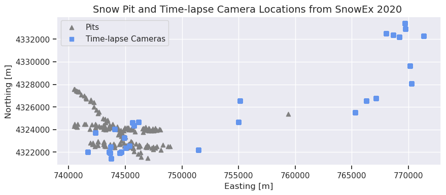
What do you notice? Is there overlap between the snow pit and camera trap locations?
Viewing the time-lapse photos
Download the sample datasets for this tutorial
For ease of access during the hackweek, sample files are available for download for running the command in the cell below.
%%bash

# Retrieve a copy of data files used in this tutorial from Zenodo.org:
# Re-running this cell will not re-download things if they already exist

mkdir -p /tmp/tutorial-data
cd /tmp/tutorial-data
wget -q -nc -O data.zip https://zenodo.org/record/5504396/files/camera-trap.zip
unzip -q -n data.zip
rm data.zip
TUTORIAL_DATA = '/tmp/tutorial-data/camera-trap'
Important Note :class: hint
Remember, this is a subset of sample images from SnowEx 2020 temporarily stored for SnowEx Hackweek The final images for SnowEx 2017 and 2020 will all be available on NSIDC.
Now display an example time-lapse image inside the notebook
We will now pull time-lapse imagery for one camera, camera E9B, from the SnowEx 2020 field campaign. E9B is from the E ast side of the Mesa, in a high vegetation area (9), and it is the second replicate of this combination (B). We will pull images and display a sample from various times of the winter season to provide a sense of what image and the snow poles look like.
# Pull and display the images from Oct, Jan, and May
october_img = Image(filename=f'{TUTORIAL_DATA}/WSCT0101.JPG', width=500, height=350)
print('Site E9B in October')
display(october_img)

january_img = Image(filename=f'{TUTORIAL_DATA}/WSCT0378.JPG', width=500, height=350)
print('Site E9B in January')
display(january_img)

may_img = Image(filename=f'{TUTORIAL_DATA}/WSCT0742.JPG', width=500, height=350)
print('Site E9B in May')
display(may_img)
Site E9B in October

Site E9B in January

Site E9B in May

What do you notice? Is this an open or closed canopy site?
Can you see the snow rising and falling on the pole?
What are some snow properties that you might be able to measure using these devices?
Time-lapse Camera Applications
1. Snow Depth from Time-lapse Images
Installing snow poles in front of time-lapse camera provides low-cost, long-term snow depth timeseries. Snow depths from the 2020 SnowEx time-lapse imagery have been manually processed with estimation of submission to the NSIDC database in summer 2021.
The snow depth is the difference between the number of pixels in a snow-free image and an image with snow, with a conversion from pixels to centimeters (Figure 1).
pil_img = Image(filename=f'{TUTORIAL_DATA}/Picture1.png', width=800, height=500)
display(pil_img)
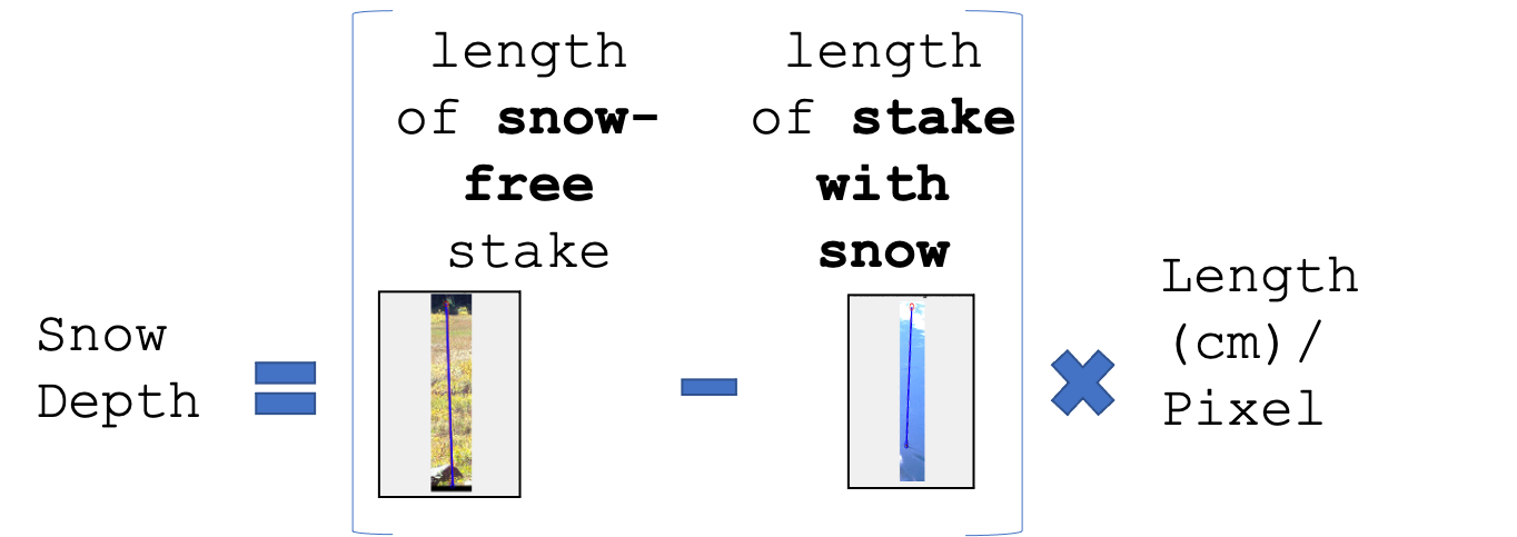
Figure 1: Equation to extract snow depth from camera images. For each image, take the difference in pixels between the length of a snow-free stake and the length of the stake and multiply by length(cm)/pixel. The ratio can be found by dividing the full length of the stake (304.8 cm) by the length of a snow-free stake in pixels.
Below we will explore the snow depth dataset created from this methodology.
Plot the Snow Depth created from a Vegetated and an Open Camera Site
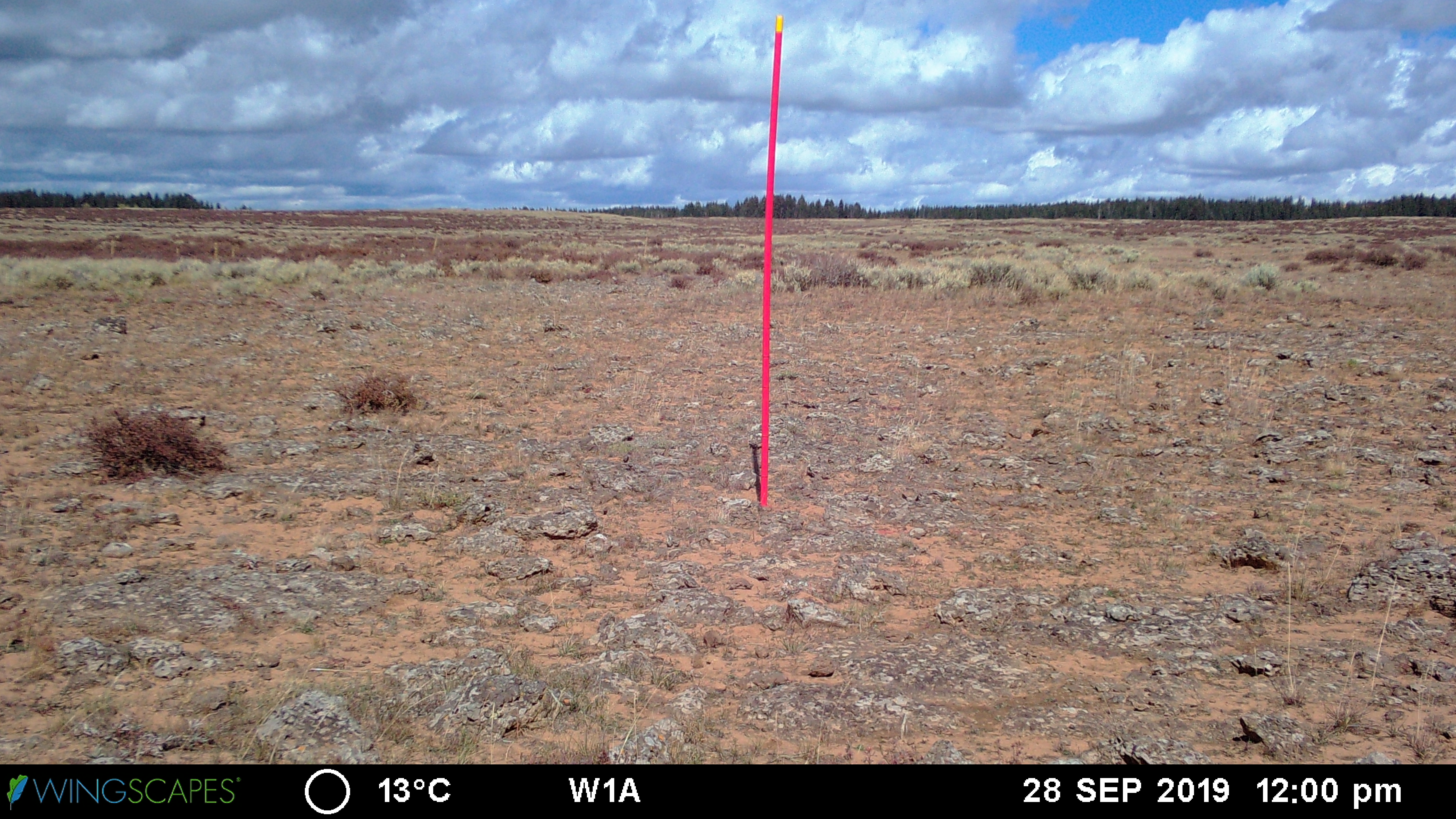
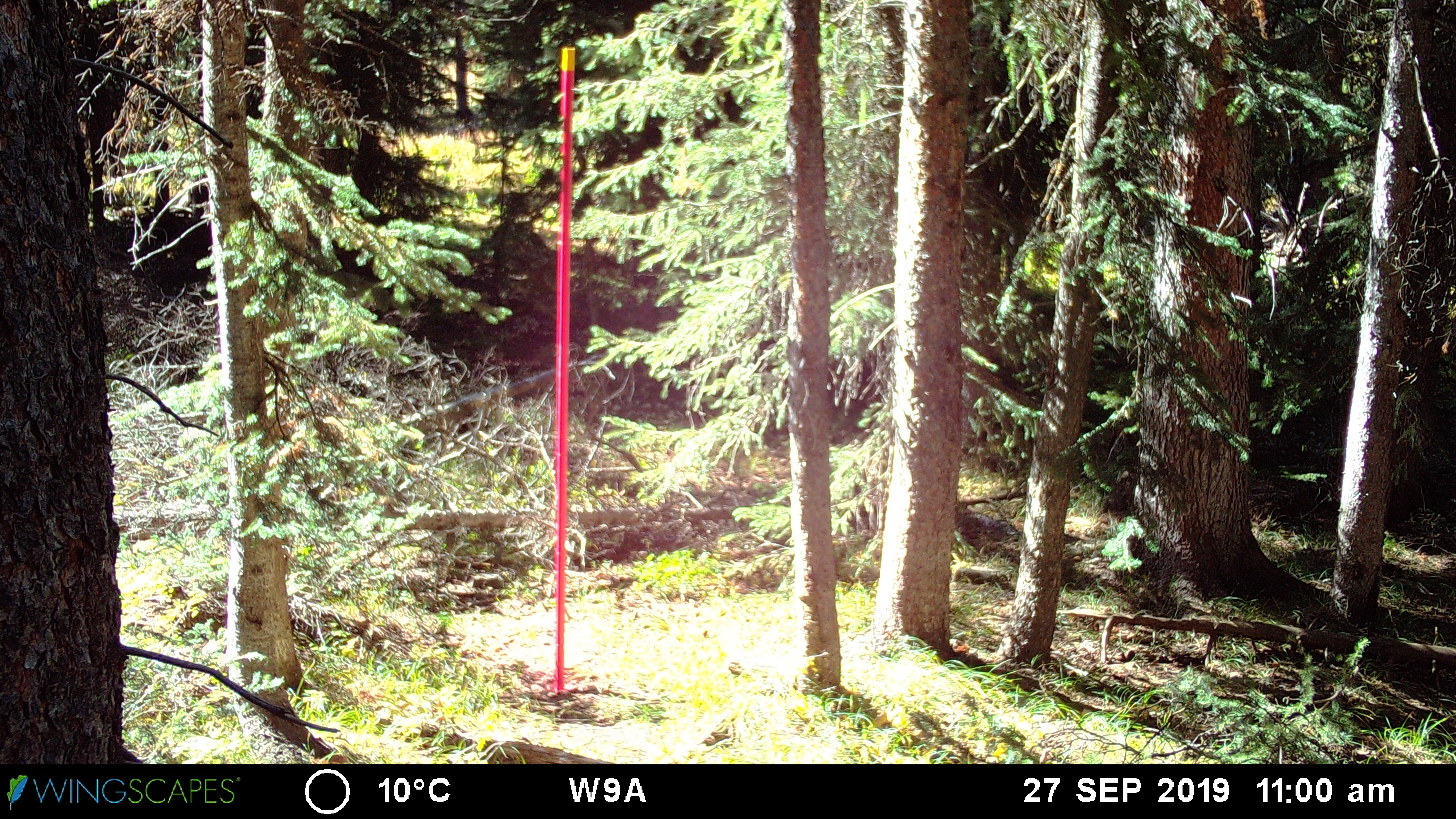
The SnowEx SQL database that we used to plot the locations has the snow depth values at all cameras. To show how we can use the SQL database to plot depths at different cameras, we will compare two cameras on the same (West) side of the Mesa, cameras W1A and W9A. One is an open site (W1A) and the other is a closed site (W9A).
Let’s start by visualizing where these two camera sites are on Grand Mesa
This is an interactive plot. You can zoom into the sites and click on the location icon to see the site name.
\(\color{blue}{\text{W1A: Open Site in blue}}\)
\(\color{green}{\text{W9A: Forested Site in green}}\)
# Create the folium map, more folium package information here: https://python-visualization.github.io/folium/modules.html
m = folium.Map(location=[39.035, -108.1612], tiles="Stamen Terrain", zoom_start=12, width='60%', height='60%', control_scale=True) # location (lat,lon) are the map center, tiles is the base map
folium.Marker([39.017236,-108.18488], popup="W1A: Open Site", tooltip=tooltip, icon=folium.Icon(color='darkblue')).add_to(m) # add a marker for W1A: Open Site in Blue
folium.Marker([39.036208,-108.161851], popup="W9A: Forested Site", tooltip=tooltip, icon=folium.Icon(color='darkgreen')).add_to(m) # add a marker for W9A: Forested Site in Green
m # Plot the final map
View associated time-lapse images using the AWS server.
open_canopy = Image(filename=f'{TUTORIAL_DATA}/W1A/WSCT0013.JPG',  width=500, height=350)
print('Below is the open site, W1A')
display(open_canopy)
closed_canopy = Image(filename=f'{TUTORIAL_DATA}/W9A/WSCT0009.JPG',  width=500, height=350)
print('Below is the forested site, W9A')
display(closed_canopy)
Below is the open site, W1A
Below is the forested site, W9A
Grab the site data for both sites from the database
# Grab the open site data from the database
open_site = 'W1A'
veg_site = 'W9A'
qry = session.query(PointData).filter(PointData.equipment.contains(open_site))
df_open = query_to_geopandas(qry,engine)

# Grab the vegetated site from the database
qry = session.query(PointData).filter(PointData.equipment.contains(veg_site))
df_veg = query_to_geopandas(qry,engine)

# Set the date as the index for easy plotting/reading
df_open = df_open.set_index('date')
df_veg = df_veg.set_index('date')
Plot the snow depth from open and forested time-lapse camera sites together
# Plot the two datasets by date
ax = df_open['value'].plot(label=f'Open Site ({open_site})', color='royalblue', linewidth=2) #  'value' column is snow depth column in SQL database
df_veg['value'].plot(ax=ax, label=f'Forested Site ({veg_site})', color='green', linewidth=2) #  'value' column is snow depth column in SQL database

# Mess with some labeling to make it look nice
ax.legend()
ax.set_ylabel('Snow Depth [cm]')

plt.title('Snow Depth for Water Year (WY) 2020 from Two Different Time-lapse Camera Locations')
plt.tight_layout()
plt.grid()
plt.show()
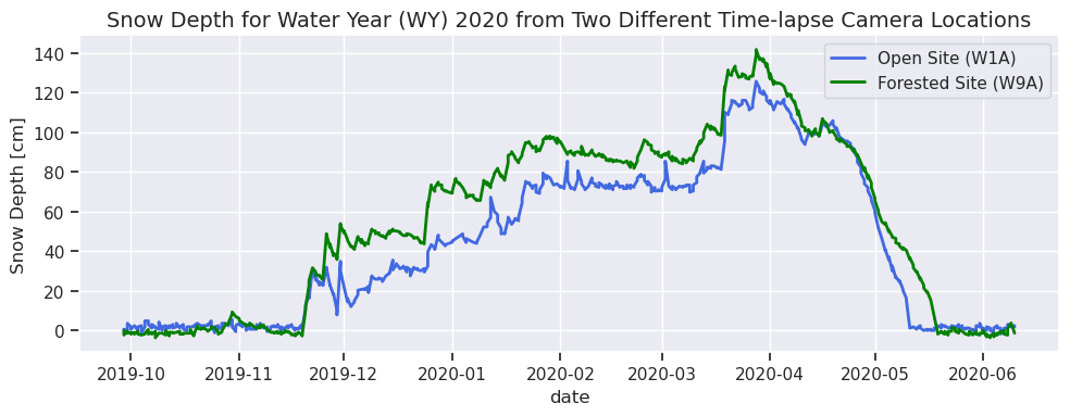
Previous forest-snow research, such as Dickerson-Lange et al. (2017), have used similar analysis to determine the snow disappearance timing in forested regions of the Pacific Northwest. Further research could use this dataset to explore the following,
What do you notice about the differences between the open and closed canopy site?
What might be some drawbacks to this method?
What would it look like to map and compare snow depth at all the closed canopy sites to all the open canopy sites?
2. Citizen Science Snow Classifications
Time-lapse photos from SnowEx 2017 were uploaded to a citizen science platform called Zooniverse (https://www.zooniverse.org/) and classified by thousands of volunteers as part of the Snow Spotter project (https://www.zooniverse.org/projects/mozerm/snow-spotter). Citizen scientists responded to questions about snow in the time-lapse photos, such as “is there snow on the ground?”, “is there snow in the tree branches?” and “are there clouds in the sky?”. These classifications are used to create a binary timeseries about snow conditions at the time-lapse camera sites on Grand Mesa for 2017 (in review Lumbrazo et al., 2021).
The 2020 images will be uploaded to Snow Spotter and classified by citizen scientists as well.
Potential Project Ideas
Compare snow depth created from the snow poles with >1 additional SnowEx snow depth measurement
snow pit snow depth data, airborne LiDAR, snow depth from ground-based terrestrial lidar, etc.
Compare snow depths created from the snow poles between open and closed vegetation sites
Pull in sample time-lapse images for sites you are working with to view the canopy conditions and visualize site characteristics
If you have any other questions or ideas throughout Hackweek, we will be happy to help! Feel free to contact us.
Tutorial Authors
Catherine (Katie) Breen, cbreen@uw.edu
Cassie Wells Lumbrazo, lumbraca@uw.edu
If you want to use any time-lapse photos for your Hackweek projects, the following are on the SnowEx’s Amazon Web Service (AWS) server for easy downloading this week,
All the time-lapse photos from two 2020 sites (i.e., W1A, W9A)
1 photo from every 2020 time-lapse camera site (images from early-February)
And everything else will be available on NSIDC.
Thanks for attending this tutorial. We look forward to see what you will find in these datasets!
Acknowledgements: Anthony Arendt, Scott Henderson, Micah Johnson, Carrie Vuyovich, Ryan Currier, Megan Mason, Mark Raleigh
Additional notes
Automated methods to extract snow depth using the Hough Transform (Currier et al. 2017) have been used on this (in progress Breen et al., 2021). The available automated and manual codes are available on GitHub: https://github.com/wcurrier/Measure_Snow_Depth_Poles & https://github.com/catherine-m-breen/Snow-Depth-From-Snow-Stakes.
References
Dickerson-Lange et al., 2017. Snow disappearance timing is dominated by forest effects on snow accumulation in warm winter climates of the Pacific Northwest, United States. Hydrological Processes. Vol 31, Issue 10. 13 February 2017. https://doi.org/10.1002/hyp.11144
Raleigh et al., 2013. Approximating snow surface temperature from standard temperature and humidity data: New possibilities for snow model and remote sensing evaluation. Water Resources Research. Vol 49, Issue 12. 07 November 2013. https://doi.org/10.1002/2013WR013958