Dynamic Query of SNOTEL data¶

SnowEx Hackweek
July 13, 2021

Author: David Shean

Introduction¶

This tutorial will demonstrate a subset of basic concepts of geospatial data processing and analysis using data from the SNOTEL sensor network. We will demonstrate dynamic query of a public API to fetch point location data, review coordinate system transformations with GeoPandas, Geometry objects, and Pandas time series analysis/visualization.

Read a bit about SNOTEL data for the Western U.S.¶

https://www.wcc.nrcs.usda.gov/snow/

This is actually a nice web interface, with some advanced querying and interactive visualization. You can also download formatted ASCII files (csv) for analysis. This is great for one-time projects, but it’s nice to have reproducible code that can be updated as new data appear, without manual steps. That’s what we’re going to do here.

About SNOTEL sites and data:¶

Sample plots for SNOTEL site at Paradise, WA (south side of Mt. Rainier)¶

https://www.nwrfc.noaa.gov/snow/snowplot.cgi?AFSW1
We will reproduce some of these plots/metrics in this tutorial

Interactive dashboard¶

https://climate.washington.edu/climate-data/snowdepth/

Snow today¶

https://nsidc.org/reports/snow-today

CUAHSI WOF server and automated Python data queries¶

We are going to use a server set up by CUAHSI to serve the SNOTEL data, using a standardized database storage format and query structure. You don’t need to worry about this, but can quickly review the following:

#This is the latest CUAHSI API endpoint
wsdlurl = 'https://hydroportal.cuahsi.org/Snotel/cuahsi_1_1.asmx?WSDL'

Acronym soup¶

SNOTEL = Snow Telemetry
CUAHSI = Consortium of Universities for the Advancement of Hydrologic Science, Inc
WOF = WaterOneFlow
WSDL = Web Services Description Language
USDA = United States Department of Agriculture
NRCS = National Resources Conservation Service
AWDB = Air-Water Database

Python options¶

There are a few packages out there that offer convenience functions to query the online SNOTEL databases and unpack the results.

climata (https://pypi.org/project/climata/) - last commit Sept 2017 (not a good sign)
ulmo (https://github.com/ulmo-dev/ulmo) - maintained by Emilio Mayorga over at UW APL)

You can also write your own queries using the Python requests module and some built-in XML parsing libraries.

Hopefully not overwhelming amount of information - let’s just go with ulmo for now. I’ve done most of the work to prepare functions for querying and processing the data. Once you wrap your head around all of the acronyms, it’s pretty simple, basically running a few functions here: https://ulmo.readthedocs.io/en/latest/api.html#module-ulmo.cuahsi.wof

We will use ulmo with daily data for this exercise, but please feel free to experiment with hourly data, other variables or other approaches to fetch SNOTEL data.

import os
from datetime import datetime
import numpy as np
import matplotlib.pyplot as plt
import pandas as pd
import geopandas as gpd
from shapely.geometry import Point
import contextily as ctx
import ulmo

Part 1: Spatial Query SNOTEL sites¶

Use the ulmo cuahsi interface and the get_sites function to fetch available site metadata from server
This will return a Python dictionary

sites = ulmo.cuahsi.wof.get_sites(wsdlurl)

#Preview first item in dictionary
next(iter(sites.items()))

('SNOTEL:301_CA_SNTL',
 {'code': '301_CA_SNTL',
  'name': 'Adin Mtn',
  'network': 'SNOTEL',
  'location': {'latitude': '41.2358283996582',
   'longitude': '-120.79192352294922'},
  'elevation_m': '1886.7120361328125',
  'site_property': {'county': 'Modoc',
   'state': 'California',
   'site_comments': 'beginDate=10/1/1983 12:00:00 AM|endDate=1/1/2100 12:00:00 AM|HUC=180200021403|HUD=18020002|TimeZone=-8.0|actonId=20H13S|shefId=ADMC1|stationTriplet=301:CA:SNTL|isActive=True',
   'pos_accuracy_m': '0'}})

Store the dictionary as a Pandas DataFrame called `sites_df`¶

See the Pandas from_dict function
Use orient option so the sites comprise the DataFrame index, with columns for ‘name’, ‘elevation_m’, etc
Use the dropna method to remove any empty records

sites_df = pd.DataFrame.from_dict(sites, orient='index').dropna()
sites_df.head()

	code	name	network	location	elevation_m	site_property
SNOTEL:301_CA_SNTL	301_CA_SNTL	Adin Mtn	SNOTEL	{'latitude': '41.2358283996582', 'longitude': ...	1886.7120361328125	{'county': 'Modoc', 'state': 'California', 'si...
SNOTEL:907_UT_SNTL	907_UT_SNTL	Agua Canyon	SNOTEL	{'latitude': '37.522171020507813', 'longitude'...	2712.719970703125	{'county': 'Kane', 'state': 'Utah', 'site_comm...
SNOTEL:916_MT_SNTL	916_MT_SNTL	Albro Lake	SNOTEL	{'latitude': '45.59722900390625', 'longitude':...	2529.840087890625	{'county': 'Madison', 'state': 'Montana', 'sit...
SNOTEL:1267_AK_SNTL	1267_AK_SNTL	Alexander Lake	SNOTEL	{'latitude': '61.749668121337891', 'longitude'...	48.768001556396484	{'county': 'Matanuska-Susitna', 'state': 'Alas...
SNOTEL:908_WA_SNTL	908_WA_SNTL	Alpine Meadows	SNOTEL	{'latitude': '47.779571533203125', 'longitude'...	1066.800048828125	{'county': 'King', 'state': 'Washington', 'sit...

Clean up the DataFrame and prepare Point geometry objects¶

Convert 'location' column (contains dictionary with 'latitude' and 'longitude' values) to Shapely Point objects
Store as a new 'geometry' column (needed by GeoPandas)
Drop the 'location' column, as this is no longer needed
Update the dtype of the 'elevation_m' column to float

sites_df['geometry'] = [Point(float(loc['longitude']), float(loc['latitude'])) for loc in sites_df['location']]

sites_df = sites_df.drop(columns='location')
sites_df = sites_df.astype({"elevation_m":float})

Review output¶

Take a moment to familiarize yourself with the DataFrame structure and different columns.
Note that the index is a set of strings with format ‘SNOTEL:1000_OR_SNTL’
Extract the first record with loc
- Review the 'site_property' dictionary - could parse this and store as separate fields in the DataFrame if desired

sites_df.head()

	code	name	network	elevation_m	site_property	geometry
SNOTEL:301_CA_SNTL	301_CA_SNTL	Adin Mtn	SNOTEL	1886.712036	{'county': 'Modoc', 'state': 'California', 'si...	POINT (-120.7919235229492 41.2358283996582)
SNOTEL:907_UT_SNTL	907_UT_SNTL	Agua Canyon	SNOTEL	2712.719971	{'county': 'Kane', 'state': 'Utah', 'site_comm...	POINT (-112.2711791992188 37.52217102050781)
SNOTEL:916_MT_SNTL	916_MT_SNTL	Albro Lake	SNOTEL	2529.840088	{'county': 'Madison', 'state': 'Montana', 'sit...	POINT (-111.9590225219727 45.59722900390625)
SNOTEL:1267_AK_SNTL	1267_AK_SNTL	Alexander Lake	SNOTEL	48.768002	{'county': 'Matanuska-Susitna', 'state': 'Alas...	POINT (-150.8896636962891 61.74966812133789)
SNOTEL:908_WA_SNTL	908_WA_SNTL	Alpine Meadows	SNOTEL	1066.800049	{'county': 'King', 'state': 'Washington', 'sit...	POINT (-121.6984710693359 47.77957153320312)

sites_df.loc['SNOTEL:301_CA_SNTL']

code                                                   301_CA_SNTL
name                                                      Adin Mtn
network                                                     SNOTEL
elevation_m                                            1886.712036
site_property    {'county': 'Modoc', 'state': 'California', 'si...
geometry               POINT (-120.7919235229492 41.2358283996582)
Name: SNOTEL:301_CA_SNTL, dtype: object

sites_df.loc['SNOTEL:301_CA_SNTL']['site_property']

{'county': 'Modoc',
 'state': 'California',
 'site_comments': 'beginDate=10/1/1983 12:00:00 AM|endDate=1/1/2100 12:00:00 AM|HUC=180200021403|HUD=18020002|TimeZone=-8.0|actonId=20H13S|shefId=ADMC1|stationTriplet=301:CA:SNTL|isActive=True',
 'pos_accuracy_m': '0'}

Convert to a Geopandas GeoDataFrame¶

We already have 'geometry' column, but still need to define the crs of the point coordinates
Note the number of records

sites_gdf_all = gpd.GeoDataFrame(sites_df, crs='EPSG:4326')
sites_gdf_all.head()

	code	name	network	elevation_m	site_property	geometry
SNOTEL:301_CA_SNTL	301_CA_SNTL	Adin Mtn	SNOTEL	1886.712036	{'county': 'Modoc', 'state': 'California', 'si...	POINT (-120.79192 41.23583)
SNOTEL:907_UT_SNTL	907_UT_SNTL	Agua Canyon	SNOTEL	2712.719971	{'county': 'Kane', 'state': 'Utah', 'site_comm...	POINT (-112.27118 37.52217)
SNOTEL:916_MT_SNTL	916_MT_SNTL	Albro Lake	SNOTEL	2529.840088	{'county': 'Madison', 'state': 'Montana', 'sit...	POINT (-111.95902 45.59723)
SNOTEL:1267_AK_SNTL	1267_AK_SNTL	Alexander Lake	SNOTEL	48.768002	{'county': 'Matanuska-Susitna', 'state': 'Alas...	POINT (-150.88966 61.74967)
SNOTEL:908_WA_SNTL	908_WA_SNTL	Alpine Meadows	SNOTEL	1066.800049	{'county': 'King', 'state': 'Washington', 'sit...	POINT (-121.69847 47.77957)

sites_gdf_all.shape

(930, 6)

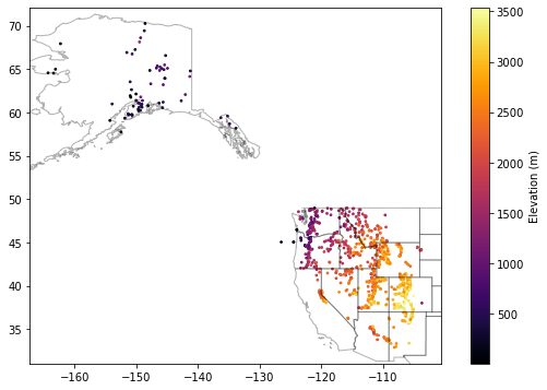
Create a scatterplot showing elevation values for all sites¶

#geojson of state polygons
states_url = 'http://eric.clst.org/assets/wiki/uploads/Stuff/gz_2010_us_040_00_5m.json'
states_gdf = gpd.read_file(states_url)

f, ax = plt.subplots(figsize=(10,6))
sites_gdf_all.plot(ax=ax, column='elevation_m', markersize=3, cmap='inferno', legend=True, legend_kwds={'label': "Elevation (m)"})
#This prevents matplotlib from updating the axes extent (states polygons cover larger area than SNOTEL points)
ax.autoscale(False)
states_gdf.plot(ax=ax, facecolor='none', edgecolor='k', alpha=0.3);

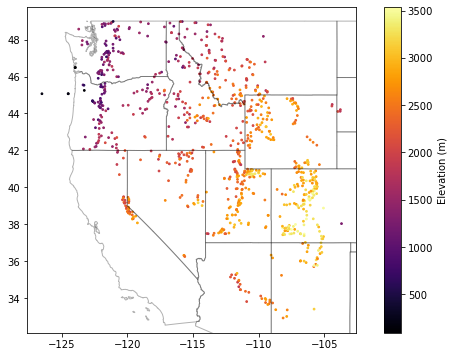
Exclude the Alaska (AK) points to isolate points over Western U.S.¶

Simple appraoch is to remove points where the site name contains ‘AK’ with attribute filter
Note the number of records

sites_gdf_conus = sites_gdf_all[~(sites_gdf_all.index.str.contains('AK'))]

Alternatively, can use a spatial filter (see GeoPandas cx indexer functionality for a bounding box)

#xmin, xmax, ymin, ymax = [-126, 102, 30, 50]
#sites_gdf_conus = sites_gdf_all.cx[xmin:xmax, ymin:ymax]

sites_gdf_conus.shape

(865, 6)

Update your scatterplot as sanity check¶

Should look something like the Western U.S.

f, ax = plt.subplots(figsize=(10,6))
sites_gdf_conus.plot(ax=ax, column='elevation_m', markersize=3, cmap='inferno', legend=True, legend_kwds={'label': "Elevation (m)"})
ax.autoscale(False)
states_gdf.plot(ax=ax, facecolor='none', edgecolor='k', alpha=0.3);

Export SNOTEL site GeoDataFrame as a geojson¶

Maybe useful for other purposes, and can avoid all of the above processing, just load directly with geopandas read_file

sites_gdf_conus.to_file?

sites_fn = 'snotel_conus_sites.json'
if not os.path.exists(sites_fn):
    sites_gdf_conus.to_file(sites_fn, driver='GeoJSON')

Part 2: Spatial filter points by polygon¶

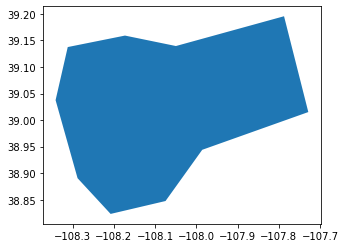
Load Grand Mesa Polygon¶

gm_poly_fn = 'grand_mesa_poly.geojson'

gm_poly_gdf = gpd.read_file(gm_poly_fn)

gm_poly_gdf.plot()

<AxesSubplot:>

A quick aside on `geometry` objects¶

Vector data contain `geometry` objects¶

Classes (Point, Line, Polygon) with unique attribute and methods
Polygon vs. MultiPolygon
https://automating-gis-processes.github.io/site/notebooks/L1/geometric-objects.html
https://shapely.readthedocs.io/en/stable/manual.html#geometric-objects

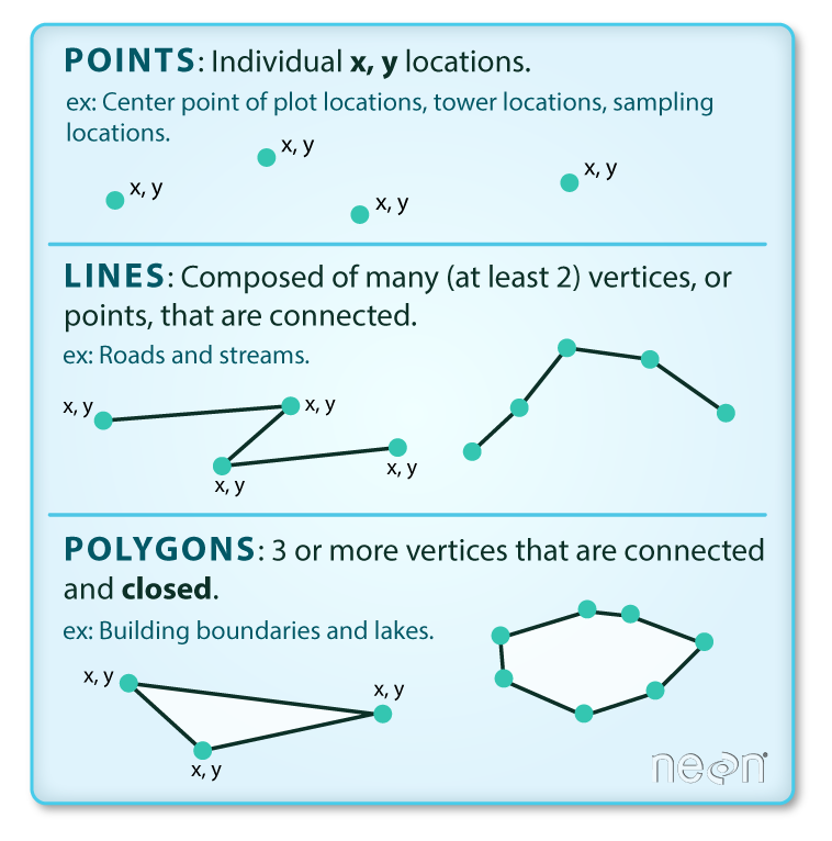Geometry types Image Source: National Ecological Observatory Network (NEON), from https://datacarpentry.org/organization-geospatial

Isolate Polygon geometry within GeoDataFrame¶

type(gm_poly_gdf)

geopandas.geodataframe.GeoDataFrame

gm_poly_gdf

	geometry
0	POLYGON ((-108.31168 39.13758, -108.34116 39.0...

gm_poly_gdf.total_bounds

array([-108.34115668,   38.82320553, -107.72839859,   39.19563035])

gm_poly_gdf.iloc[0] #Now a GeoSeries

geometry    POLYGON ((-108.31168 39.13758, -108.34116 39.0...
Name: 0, dtype: geometry

gm_poly_geom = gm_poly_gdf.iloc[0].geometry
gm_poly_geom

print(gm_poly_geom)

POLYGON ((-108.3116825655377 39.13757646212944, -108.3411566832522 39.03758987613325, -108.2878686387796 38.89051431295789, -108.2077296878005 38.8232055291981, -108.0746016431103 38.8475137825863, -107.9856051049498 38.9439912011017, -107.7283985875575 39.01510930230633, -107.7872414249099 39.19563034965999, -108.0493948009875 39.13950466335424, -108.1728700097086 39.15920066396116, -108.3116825655377 39.13757646212944))

list(gm_poly_geom.exterior.coords)

[(-108.31168256553767, 39.13757646212944),
 (-108.34115668325224, 39.03758987613325),
 (-108.2878686387796, 38.89051431295789),
 (-108.20772968780051, 38.8232055291981),
 (-108.07460164311031, 38.8475137825863),
 (-107.98560510494981, 38.9439912011017),
 (-107.72839858755752, 39.01510930230633),
 (-107.78724142490994, 39.195630349659986),
 (-108.04939480098754, 39.139504663354245),
 (-108.17287000970857, 39.15920066396116),
 (-108.31168256553767, 39.13757646212944)]

gm_poly_geom.bounds

(-108.34115668325224,
 38.8232055291981,
 -107.72839858755752,
 39.195630349659986)

Generate boolean index for points that intersect the polygon¶

This will return a new GeoDataSeries with True/False values for each record

idx = sites_gdf_all.intersects(gm_poly_geom)

idx.head()

SNOTEL:301_CA_SNTL     False
SNOTEL:907_UT_SNTL     False
SNOTEL:916_MT_SNTL     False
SNOTEL:1267_AK_SNTL    False
SNOTEL:908_WA_SNTL     False
dtype: bool

idx.value_counts()

False    928
True       2
dtype: int64

Use fancy indexing to isolate points and return new GeoDataFrame¶

gm_snotel_sites = sites_gdf_all.loc[idx]

gm_snotel_sites

	code	name	network	elevation_m	site_property	geometry
SNOTEL:622_CO_SNTL	622_CO_SNTL	Mesa Lakes	SNOTEL	3048.000000	{'county': 'Mesa', 'state': 'Colorado', 'site_...	POINT (-108.05835 39.05831)
SNOTEL:682_CO_SNTL	682_CO_SNTL	Park Reservoir	SNOTEL	3035.808105	{'county': 'Delta', 'state': 'Colorado', 'site...	POINT (-107.87414 39.04644)

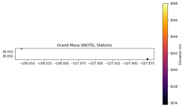
Quick plot¶

f, ax = plt.subplots(figsize=(10,6))
gm_snotel_sites.plot(ax=ax, column='elevation_m', markersize=20, edgecolor='k', cmap='inferno', \
                  legend=True, legend_kwds={'label':'Elevation (m)'})
#ctx.add_basemap(ax=ax, crs=gm_snotel_sites.crs, source=ctx.providers.Stamen.Terrain)
ax.set_title('Grand Mesa SNOTEL Stations');

import hvplot.pandas
from geoviews import tile_sources as gvts

gm_snotel_sites.hvplot(hover_cols=['index','name']) * gm_poly_gdf.to_crs(gm_snotel_sites.crs).hvplot(color='none')

Add a basemap¶

This functionality will add a publicly available tiled basemap to your interactive holoviews plot, which is useful for context during interactive visualization.

Note that we need to reproject our GeoDataframe to match the CRS of the tiled basemap here.

For static plots with matplotlib (e.g., for publication) can also use contextily for this https://contextily.readthedocs.io/en/latest/

map_tiles = gvts.EsriImagery

map_tiles * gm_snotel_sites.to_crs('EPSG:3857').hvplot(hover_cols=['index','name']) * \
gm_poly_gdf.to_crs('EPSG:3857').hvplot(color='none')

Part 3: Time series analysis for one station¶

Now that we’ve identified sites of interest, let’s query the API to obtain the time series data for variables of interest (snow!).

https://wcc.sc.egov.usda.gov/nwcc/site?sitenum=622&state=co

sitecode = gm_snotel_sites.index[-1]
sitecode

'SNOTEL:682_CO_SNTL'

Get available measurements for this site¶

Note that there are many standard meteorological variables that can be downloaded for this site, in addition to the snow depth and snow water equivalent.

ulmo.cuahsi.wof.get_site_info(wsdlurl, sitecode)['series'].keys()

dict_keys(['SNOTEL:BATT_D', 'SNOTEL:BATT_H', 'SNOTEL:BATX_H', 'SNOTEL:PRCP_y', 'SNOTEL:PRCP_sm', 'SNOTEL:PRCP_m', 'SNOTEL:PRCP_wy', 'SNOTEL:PRCPSA_y', 'SNOTEL:PRCPSA_D', 'SNOTEL:PRCPSA_sm', 'SNOTEL:PRCPSA_m', 'SNOTEL:PRCPSA_wy', 'SNOTEL:PREC_sm', 'SNOTEL:PREC_m', 'SNOTEL:PREC_wy', 'SNOTEL:SNWD_D', 'SNOTEL:SNWD_sm', 'SNOTEL:SNWD_H', 'SNOTEL:SNWD_m', 'SNOTEL:TAVG_y', 'SNOTEL:TAVG_D', 'SNOTEL:TAVG_sm', 'SNOTEL:TAVG_m', 'SNOTEL:TAVG_wy', 'SNOTEL:TMAX_y', 'SNOTEL:TMAX_D', 'SNOTEL:TMAX_sm', 'SNOTEL:TMAX_m', 'SNOTEL:TMAX_wy', 'SNOTEL:TMIN_y', 'SNOTEL:TMIN_D', 'SNOTEL:TMIN_sm', 'SNOTEL:TMIN_m', 'SNOTEL:TMIN_wy', 'SNOTEL:TOBS_D', 'SNOTEL:TOBS_sm', 'SNOTEL:TOBS_H', 'SNOTEL:TOBS_m', 'SNOTEL:WTEQ_D', 'SNOTEL:WTEQ_sm', 'SNOTEL:WTEQ_H', 'SNOTEL:WTEQ_m'])

_H = “hourly”
_D = “daily”
_sm, _m = “monthly”

Let’s consider the ‘SNOTEL:SNWD_D’ variable (Daily Snow Depth)¶

Assign ‘SNOTEL:SNWD_D’ to a variable named variablecode
Get some information about the variable using get_variable_info method
- Note the units, nodata value, etc.
Note: The snow depth records are almost always shorter/noisier than the SWE records for SNOTEL sites

#Daily SWE
#variablecode = 'SNOTEL:WTEQ_D'
#Daily snow depth
variablecode = 'SNOTEL:SNWD_D'

#Hourly SWE
#variablecode = 'SNOTEL:WTEQ_H'
#Hourly snow depth
#variablecode = 'SNOTEL:SNWD_H'

ulmo.cuahsi.wof.get_variable_info(wsdlurl, variablecode)

{'value_type': 'Field Observation',
 'data_type': 'Continuous',
 'general_category': 'Soil',
 'sample_medium': 'Snow',
 'no_data_value': '-9999',
 'speciation': 'Not Applicable',
 'code': 'SNWD_D',
 'id': '176',
 'name': 'Snow depth',
 'vocabulary': 'SNOTEL',
 'time': {'is_regular': True,
  'interval': '1',
  'units': {'abbreviation': 'd',
   'code': '104',
   'name': 'day',
   'type': 'Time'}},
 'units': {'abbreviation': 'in',
  'code': '49',
  'name': 'international inch',
  'type': 'Length'}}

Define a function to fetch data¶

I’ve done this for you, but please review the comments and steps to see what is going on under the hood
You’ll probably have to do similar data wrangling for another project at some point in the future

#Get current datetime
today = datetime.today().strftime('%Y-%m-%d')

def snotel_fetch(sitecode, variablecode='SNOTEL:SNWD_D', start_date='1950-10-01', end_date=today):
    #print(sitecode, variablecode, start_date, end_date)
    values_df = None
    try:
        #Request data from the server
        site_values = ulmo.cuahsi.wof.get_values(wsdlurl, sitecode, variablecode, start=start_date, end=end_date)
        #Convert to a Pandas DataFrame   
        values_df = pd.DataFrame.from_dict(site_values['values'])
        #Parse the datetime values to Pandas Timestamp objects
        values_df['datetime'] = pd.to_datetime(values_df['datetime'], utc=True)
        #Set the DataFrame index to the Timestamps
        values_df = values_df.set_index('datetime')
        #Convert values to float and replace -9999 nodata values with NaN
        values_df['value'] = pd.to_numeric(values_df['value']).replace(-9999, np.nan)
        #Remove any records flagged with lower quality
        values_df = values_df[values_df['quality_control_level_code'] == '1']
    except:
        print("Unable to fetch %s" % variablecode)

    return values_df

Use this function to get the full ‘SNOTEL:SNWD_D’ record for one station¶

Inspect the results
We used a dummy start date of Jan 1, 1950. What is the actual the first date returned?

#Get all records, can filter later
start_date = datetime(1950,1,1)
end_date = datetime.today()

print(sitecode)
values_df = snotel_fetch(sitecode, variablecode, start_date, end_date)
values_df.shape

SNOTEL:682_CO_SNTL

(8980, 8)

values_df.head()

	value	qualifiers	censor_code	date_time_utc	method_id	method_code	source_code	quality_control_level_code
datetime
1997-03-21 00:00:00+00:00	71.0	V	nc	1997-03-21T00:00:00	0	0	1	1
1997-03-22 00:00:00+00:00	70.0	V	nc	1997-03-22T00:00:00	0	0	1	1
1997-03-23 00:00:00+00:00	69.0	V	nc	1997-03-23T00:00:00	0	0	1	1
1997-03-24 00:00:00+00:00	68.0	V	nc	1997-03-24T00:00:00	0	0	1	1
1997-03-25 00:00:00+00:00	68.0	V	nc	1997-03-25T00:00:00	0	0	1	1

#Get number of decimal years between first and last observation
nyears = (values_df.index.max() - values_df.index.min()).days/365.25
nyears

24.583162217659137

Create a quick plot to view the time series¶

Take a moment to inspect the value column, which is where the SNWD_D values are stored
Sanity check thought question: What are the units again?

values_df.hvplot()

Compute the integer day of year (doy) and integer day of water year (dowy)¶

Can get doy for each record with df.index.dayofyear
- Can compute on the fly, but add a new column to store these values
- https://pandas.pydata.org/pandas-docs/version/0.19/generated/pandas.DatetimeIndex.dayofyear.html
For the day of water year, you’ll need to offset by 9 months, then compute day of year
- https://en.wikipedia.org/wiki/Water_year
- Add another column to store these values

#Add DOY and DOWY column
#Need to revisit for leap year support
def add_dowy(df, col=None):
    if col is None:
        df['doy'] = df.index.dayofyear
    else:
        df['doy'] = df[col].dayofyear
    # Sept 30 is doy 273
    df['dowy'] = df['doy'] - 273
    df.loc[df['dowy'] <= 0, 'dowy'] += 365

add_dowy(values_df)

Compute statistics for each day of the water year, using values from all years¶

Seems like a Pandas groupby/agg might work here
Stats should at least include min, max, mean, and median

stat_list = ['count','min','max','mean','std','median','mad']

doy_stats = values_df.groupby('dowy').agg(stat_list)['value']
doy_stats

	count	min	max	mean	std	median	mad
dowy
1	21	0.0	1.0	0.095238	0.300793	0.0	0.172336
2	21	0.0	3.0	0.285714	0.783764	0.0	0.489796
3	21	0.0	6.0	0.714286	1.454058	0.0	0.952381
4	21	0.0	10.0	0.952381	2.459191	0.0	1.360544
5	21	0.0	7.0	0.761905	1.700140	0.0	1.015873
...	...	...	...	...	...	...	...
361	20	0.0	4.0	0.400000	0.994723	0.0	0.640000
362	20	0.0	2.0	0.200000	0.523148	0.0	0.340000
363	20	0.0	2.0	0.200000	0.523148	0.0	0.340000
364	20	0.0	2.0	0.200000	0.523148	0.0	0.340000
365	20	0.0	1.0	0.050000	0.223607	0.0	0.095000

365 rows × 7 columns

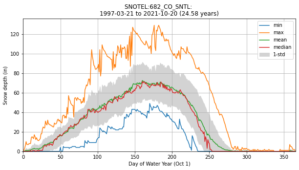
Create a plot of these aggregated dowy values¶

Something like the 30-year mean and median here: https://www.nwrfc.noaa.gov/snow/plot_SWE.php?id=AFSW1

f,ax = plt.subplots(figsize=(10,5))

for stat in ['min','max','mean','median']:
    ax.plot(doy_stats.index, doy_stats[stat], label=stat)

ax.fill_between(doy_stats.index, doy_stats['mean'] - doy_stats['std'], doy_stats['mean'] + doy_stats['std'], \
                color='lightgrey', label='1-std')

title = f'{sitecode}: \n{values_df.index.min().date()} to {values_df.index.max().date()} ({nyears:.2f} years)'

ax.set_title(title)
ax.set_xlabel('Day of Water Year (Oct 1)')
ax.set_ylabel('Snow depth (in)')
ax.grid()
ax.legend()
ax.set_xlim(0,366)
ax.set_ylim(bottom=0);

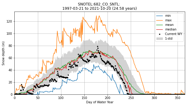
Add the daily snow depth values for the current water year¶

Can use pandas indexing here with simple strings (‘YYYY-MM-DD’), or Timestamp objects
- Standard slicing also works with :
Make sure to dropna to remove any records missing data
Add this to your plot

#Define variable to store current year
curr_y = datetime.now().year
curr_y

#df_wy = values_df.loc['2019-10-1':].dropna()
df_wy = values_df.loc[f'{curr_y-1}-10-1':].dropna()

f,ax = plt.subplots(figsize=(10,5))
for stat in ['min','max','mean','median']:
    ax.plot(doy_stats.index, doy_stats[stat], label=stat)

ax.fill_between(doy_stats.index, doy_stats['mean'] - doy_stats['std'], doy_stats['mean'] + doy_stats['std'], \
                color='lightgrey', label='1-std')

ax.set_title(title)
ax.set_xlabel('Day of Water Year')
ax.set_ylabel('Snow depth (in)')
ax.grid()
ax.plot(df_wy['dowy'], df_wy['value'], marker='.', color='k', ls='none', label='Current WY')
ax.legend()
ax.set_xlim(0,366)
ax.set_ylim(bottom=0);

What was the percentage of “normal” snow depth on April 1 of this year?¶

Can use long-term median for this dowy

df_wy.loc[f'{curr_y}-4-1']

value                                        67.0
qualifiers                                      V
censor_code                                    nc
date_time_utc                 2021-04-01T00:00:00
method_id                                       0
method_code                                     0
source_code                                     1
quality_control_level_code                      1
doy                                            91
dowy                                          183
Name: 2021-04-01 00:00:00+00:00, dtype: object

apr1_doy = df_wy.loc[f'{curr_y}-4-1']['dowy']
apr1_doy

doy_stats.loc[apr1_doy]

count      24.000000
min        42.000000
max       127.000000
mean       68.291667
std        18.892094
median     68.000000
mad        13.375000
Name: 183, dtype: float64

#Percent of normal
perc_normal = 100 * df_wy.loc[f'{curr_y}-4-1']['value']/doy_stats.loc[apr1_doy]['median']
print(f'{perc_normal:0.2f}% percent of normal snow depth on DOWY {apr1_doy} in {curr_y}')

98.53% percent of normal snow depth on DOWY 183 in 2021

Index DataFrame by date or date range¶

Maybe useful for project work

dt1 = '2017-2-1'
dt2 = '2017-2-4'

#Single date
values_df.loc[dt1]

value                                        77.0
qualifiers                                      V
censor_code                                    nc
date_time_utc                 2017-02-01T00:00:00
method_id                                       0
method_code                                     0
source_code                                     1
quality_control_level_code                      1
doy                                            32
dowy                                          124
Name: 2017-02-01 00:00:00+00:00, dtype: object

values_df.loc[dt1]['value']

77.0

values_df.loc[dt1:dt2]

	value	qualifiers	censor_code	date_time_utc	method_id	method_code	source_code	quality_control_level_code	doy	dowy
datetime
2017-02-01 00:00:00+00:00	77.0	V	nc	2017-02-01T00:00:00	0	0	1	1	32	124
2017-02-02 00:00:00+00:00	76.0	V	nc	2017-02-02T00:00:00	0	0	1	1	33	125
2017-02-03 00:00:00+00:00	76.0	V	nc	2017-02-03T00:00:00	0	0	1	1	34	126
2017-02-04 00:00:00+00:00	75.0	V	nc	2017-02-04T00:00:00	0	0	1	1	35	127

Query multiple sites¶

Can use a loop to query multiple sites and/or variables

#Define an empty dictionary to store returns for each site
value_dict = {}
for i, sitecode in enumerate(gm_snotel_sites.index):
    print('%i of %i sites: %s' % (i+1, len(gm_snotel_sites.index), sitecode))
    out = snotel_fetch(sitecode, variablecode)
    if out is not None:
        value_dict[sitecode] = out['value']
#Convert the dictionary to a DataFrame, automatically handles different datetime ranges (nice!)
multi_df = pd.DataFrame.from_dict(value_dict)

1 of 2 sites: SNOTEL:622_CO_SNTL

2 of 2 sites: SNOTEL:682_CO_SNTL

multi_df

	SNOTEL:622_CO_SNTL	SNOTEL:682_CO_SNTL
datetime
1997-03-21 00:00:00+00:00	NaN	71.0
1997-03-22 00:00:00+00:00	NaN	70.0
1997-03-23 00:00:00+00:00	NaN	69.0
1997-03-24 00:00:00+00:00	NaN	68.0
1997-03-25 00:00:00+00:00	NaN	68.0
...	...	...
2021-10-16 00:00:00+00:00	8.0	13.0
2021-10-17 00:00:00+00:00	8.0	11.0
2021-10-18 00:00:00+00:00	5.0	8.0
2021-10-19 00:00:00+00:00	NaN	8.0
2021-10-20 00:00:00+00:00	NaN	11.0

8980 rows × 2 columns

multi_df.hvplot()

#Hack to remove bad measurements
multi_df[multi_df > 190] = np.nan

multi_df.hvplot()

Scatterplot to compare corresponding values¶

multi_df.dropna().hvplot(kind='scatter', x='SNOTEL:622_CO_SNTL', y='SNOTEL:682_CO_SNTL', \
                         aspect='equal', s=1)

Determine Pearson’s correlation coefficient for the two time series¶

https://en.wikipedia.org/wiki/Pearson_correlation_coefficient
See the Pandas corr method
- This should properly handle nan under the hood!

multi_df.corr()

	SNOTEL:622_CO_SNTL	SNOTEL:682_CO_SNTL
SNOTEL:622_CO_SNTL	1.000000	0.968504
SNOTEL:682_CO_SNTL	0.968504	1.000000

Highly correlated snow depth records for these two sites!

SnowEx Hackweek